Pulse Compilers

QUASAR compiles a circuit for a star-topology device in two steps: first to the device’s native gates, then to the control pulses that realize them. A PulseCompiler performs the second step. It lowers a native gate-level circuit to hardware control pulses, for any gate set with a registered pulse backend. CROTGateSet and FixedCROTGateSet both lower to pulses on a Simphony device model, which simulates them. FixedCROTGateSet also lowers to XeedQ hardware.

You will see:

• how to benchmark every native gate on a simulated device;

• the pulse parameters a backend reads, and how to change them;

• how the measured gate errors feed the gate-level compiler;

• how the predicted error of a circuit compares with its simulated pulses;

• how a circuit compiles for XeedQ hardware.

See the Gate Compilers tutorial for how a circuit gets to native-gate form in the first place.

Setup

This notebook needs quasar and simphony, which drives the device model:

pip install --find-links=wheels/ ".[simphony-backend]"

%matplotlib inline

import quasar
import simphony
from qiskit.circuit.random import random_circuit

The device model

A default NV-center model: a nitrogen-14 nuclear spin and one nearby carbon-13, giving a 3-qubit register (electron + two nuclear spins) plus the microwave (MW_x) and radio-frequency (RF_x) driving fields that pulse compilation needs. We build it once and reuse it for the rest of the notebook.

model = simphony.default_nv_model(
    nitrogen_isotope=14,
    static_field_strength=0.05,
    carbon_atom_indices=[(2, -2, -1, 1)],
)
model

Model(spin_names=['e', 'N', 'C'], num_static_fields=1, driving_field_names=['MW_x', 'RF_x'], dimension=18)

A PulseCompiler binds a gate set to a pulse backend that’s already bound to the model.

gateset = quasar.CROTGateSet(n_qubits=3)
backend = quasar.SimphonyBackend(model=model)
pulse_compiler = quasar.PulseCompiler(gateset=gateset, backend=backend)

Benchmarking the native gates

benchmark_gateset simulates every native gate’s pulse and reports its average gate fidelity — a first look at how well the device realizes the gate set.

gate_fidelities = pulse_compiler.benchmark_gateset()
{f"{gate.gate_type.name}{gate.qubits}": fidelity for gate, fidelity in gate_fidelities.items()}

{'rz(0,)': 1.0,
 'r(0,)': 0.9990988928489162,
 'rz(1,)': 1.0,
 'r(1,)': 0.9980637857935825,
 'rz(2,)': 1.0,
 'r(2,)': 0.9947700739540777,
 'crot(0, 1)': 0.9959983650276022,
 'crot(0, 2)': 0.9935915022036217}

The gate set can carry these measured errors (see the Gate Sets tutorial). Each gate’s average infidelity, 1 - fidelity, becomes its error. The errors are known only now, after the gate set exists. with_properties returns a copy of the gate set with them, and the copy keeps every value it is not given:

gate_errors = {gate: max(0.0, 1 - fidelity) for gate, fidelity in gate_fidelities.items()}
gateset_measured = gateset.with_properties(gate_errors=gate_errors)
{f"{gate.gate_type.name}{gate.qubits}": error for gate, error in gateset_measured.gate_errors.items() if gate.gate_type.name == "crot"}

{'crot(0, 1)': 0.004001634972397805, 'crot(0, 2)': 0.00640849779637831}

Pulse parameters

The backend reads every physical number from its parameters. SimphonyBackend(model) takes the frequencies from the model. The pulse durations are choices, and the backend fills in defaults:

parameters = backend.parameters
{
    "electron pi pulse (us)": parameters.electron.strength.pi_duration,
    "decoupling pulses per DDRF sequence": parameters.n_dds,
    "RF time unit tau per nucleus (us)": {
        qubit: round(nucleus.strength.pi_duration, 2)
        for qubit, nucleus in parameters.nuclei.items()
    },
}

{'electron pi pulse (us)': 0.00676,
 'decoupling pulses per DDRF sequence': 4,
 'RF time unit tau per nucleus (us)': {1: 4.66, 2: 44.61}}

A DDRF sequence plays RF for \(\tau\) at either end, and for \(2\tau\) between two decoupling pulses.

Other values go into a PulseParameters, and every field left empty keeps its default. Here are two other operating points next to the default: a longer, weaker electron pulse, and eight decoupling pulses instead of four. benchmark_gate measures one native gate at a time:

named = {f"{gate.gate_type.name}{gate.qubits}": gate for gate in gateset.native_gates}
shown = {name: named[name] for name in ("r(0,)", "crot(0, 1)", "crot(0, 2)")}


def benchmark(candidate):
    compiler = quasar.PulseCompiler(gateset=gateset, backend=candidate)
    return {name: round(compiler.benchmark_gate(gate), 4) for name, gate in shown.items()}


electron_50_ns = quasar.PulseParameters(
    electron=quasar.DriveParameters(strength=quasar.DriveStrength(pi_duration=0.05))
)
{
    "default": benchmark(backend),
    "electron pi pulse 50 ns": benchmark(
        quasar.SimphonyBackend(model=model, parameters=electron_50_ns)
    ),
    "8 decoupling pulses": benchmark(
        quasar.SimphonyBackend(model=model, parameters=quasar.PulseParameters(n_dds=8))
    ),
}

{'default': {'r(0,)': 0.9991, 'crot(0, 1)': 0.996, 'crot(0, 2)': 0.9936},
 'electron pi pulse 50 ns': {'r(0,)': 0.9548,
  'crot(0, 1)': 0.9993,
  'crot(0, 2)': 0.9878},
 '8 decoupling pulses': {'r(0,)': 0.9991,
  'crot(0, 1)': 0.9927,
  'crot(0, 2)': 0.9983}}

Each change helps some gates and costs others. The values above are average gate fidelities:

• the longer electron pulse lowers the fidelity of the electron’s own rotation from 99.91 % to 95.48 %, and raises that of crot(0, 1) from 99.60 % to 99.93 %;

• eight decoupling pulses raise the fidelity of crot(0, 2) from 99.36 % to 99.83 %, and lower that of crot(0, 1) to 99.27 %.

The operating point is a choice for each device, and benchmark_gate measures it before any circuit runs. The rest of this notebook uses the defaults.

Compiling a circuit to pulses

To pulse-compile a whole circuit, first compile it to native gates. Here we gate-compile with the error-aware strategy on the gate set carrying the errors benchmark_gateset measured — so the gate-level compiler trades depth against this device’s real gate errors, instead of guessed values.

qc = random_circuit(num_qubits=3, depth=3, seed=6)
config_error_aware = quasar.ErrorAwareAdaptiveConfig(seed=3)
compiler_error_aware = quasar.GateCompiler(gateset_measured, config=config_error_aware)
qc_native = compiler_error_aware.compile(qc)
dict(qc_native.count_ops())

{'rz': 17, 'r': 13, 'crot': 7}

Before any pulse runs, estimate_errors predicts what the circuit will cost on this device. The physical error is the part the gates’ own errors add:

forecast = compiler_error_aware.estimate_errors(qc, qc_native)
forecast

ErrorEstimate(compilation=0.004851129848569391, physical=0.0704006303650695, overall=0.07486754728940148)

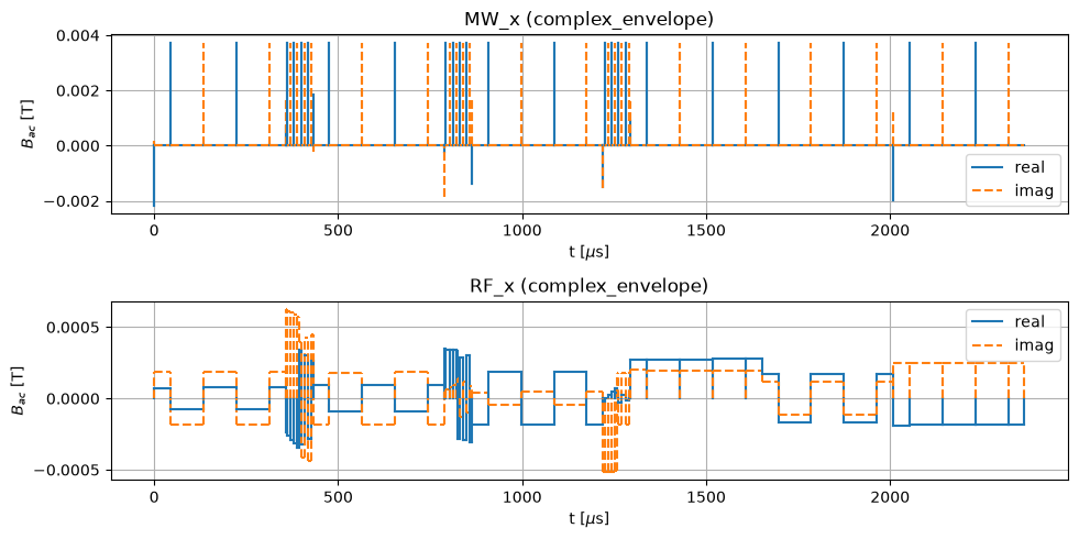
PulseCompiler.compile appends the pulses for this circuit onto the model:

pulse_compiler.compile(qc_native)

PulseList(n_pulses=116)

The resulting microwave/RF envelope:

model.plot_driving_fields(function="complex_envelope")

Finally, benchmark_circuit simulates the whole pulse sequence and compares it with the ideal native circuit. Its error is the simulated counterpart of the physical error predicted above:

fidelity = pulse_compiler.benchmark_circuit(qc_native)
{"predicted physical error": forecast.physical, "simulated error": 1 - fidelity}

{'predicted physical error': 0.0704006303650695,
 'simulated error': 0.06466949536320021}

The prediction lands close to the simulation here, slightly above it. The prediction prices every rotation at the error benchmark_gateset measured at an angle of pi/2. On this device model, a rotation’s error depends on its angle. The simulation also includes what the gates do to each other. So on another circuit, the prediction can land above or below the simulation. It is a model estimate, made before any pulse is built, so it is a quick way to compare compiled circuits for one device.

XeedQBackend: running on the real device

FixedCROTGateSet also lowers to pulses through XeedQBackend, for a real NV-center-based XeedQ quantum register. This notebook uses two of its qubits: the electron and its nitrogen-14 nucleus. It reads the calibration the device reports and emits the pulse program the device runs:

• rz is a frame change, with no pulse;

• sx on the electron is one microwave pulse;

• sx and crotxpi2 on the nucleus are a DDRF sequence: RF on the nucleus, with four microwave pulses that decouple the electron.

XeedQBackend is registered for FixedCROTGateSet, so a circuit is first gate-compiled onto that gate set, on these two qubits:

gateset_fixed = quasar.FixedCROTGateSet(n_qubits=2)
qc_xeedq = random_circuit(num_qubits=2, depth=4, seed=3)
config_adaptive = quasar.AdaptiveConfig(seed=3)
compiler_fixed = quasar.GateCompiler(gateset_fixed, config=config_adaptive)
qc_xeedq_compiled = compiler_fixed.compile(qc_xeedq)
dict(qc_xeedq_compiled.count_ops())

{'rz': 14, 'sx': 6, 'crotxpi2': 3}

With access to an XeedQ device, the backend is built from its live calibration, and the native circuit compiles to a pulse program:

xeedq_backend = quasar.XeedQBackend.from_cloud_backend(device)  # the device's cloud backend
pulse_compiler_xeedq = quasar.PulseCompiler(gateset=gateset_fixed, backend=xeedq_backend)
program = pulse_compiler_xeedq.compile(qc_xeedq_compiled)

The backend has no benchmark_* methods: benchmarking simulates the pulses against the ideal circuit, which only a simulator-backed backend can do.

Where to go next

• Qubit Layout tutorial — letting the compiler choose which qubit sits where.

• State Preparation and Pauli Readout tutorial — compiling a state preparation, a readout and a reset.

• Gate Compilers tutorial — how the gate errors shape the gate-level compile.

• The API reference for the full surface.