Gate Optimization with Autodiff

Simphony is a Python package designed for simulating the spin dynamics of point defects, in particular the nitrogen-vacancy (NV) center, which is surrounded by nuclear spins and serves as a central-spin quantum register.

This tutorial demonstrates how to leverage Simphony’s automatic differentiation (autodiff) capabilities to optimize a quantum gate at the pulse level.

We will:

• Define a physical model based on NV-center spins

• Set up an objective function using gate infidelity

• Use autodiff to compute gradients

• Apply gradient-based optimization to improve gate fidelity

Import the packages

First, enable automatic differentiation in Simphony, set the computation to run on the GPU — highly recommended for autodiff — and import the required packages:

import simphony
simphony.Config.set_platform('gpu')
simphony.Config.set_autodiff_mode(True)
simphony.Config.set_matplotlib_format('retina')

import numpy as np
import jax.numpy as jnp

from qiskit import QuantumCircuit

from matplotlib import pyplot as plt

Define the model

We use a predefined NV-center model from Simphony, which includes the electron spin and the nitrogen nuclear spin, but no carbon nuclear spins:

model = simphony.default_nv_model(nitrogen_isotope = 14,
                                  static_field_strength = 0.005)
model.plot_levels()
model.spin_names

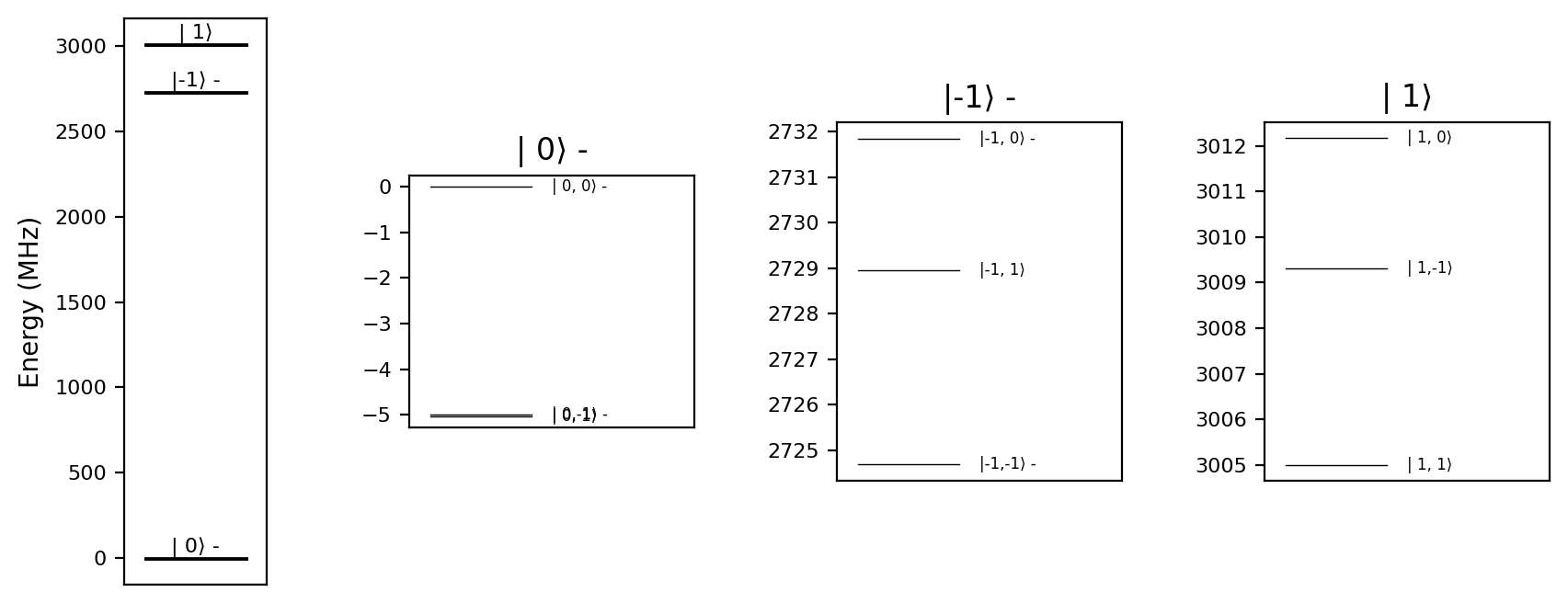
['e', 'N']

Infidelity as the Objective Function

To perform autodiff, we first define an objective function as a Python function. Infidelity quantifies how far the implemented gate deviates from the target ideal gate, making it a natural choice for the objective function.

We start by implementing an \(RX(\pi/2)\) gate on the electron spin using a resonant pulse with a rectangular envelope. Since the electron spin splitting depends on the state of the nitrogen nuclear spin, we set the driving frequency to the average electron spin splitting across nuclear spin states. The pulse duration will be treated as the optimization variable, while the amplitude is set to achieve a \(\pi/2\) rotation — corresponding to a quarter of a Rabi oscillation:

frequency = model.splitting_qubit(spin_name='e')
qc = QuantumCircuit(2)
qc.rx(np.pi/2,0)

def infidelity(duration, model):

    period_time = 4 * duration # 4 -> pi/2 gate
    amplitude = model.rabi_cycle_amplitude_qubit(driving_field_name = 'MW_x',
                                                 spin_name = 'e', 
                                                 period_time = period_time)
    
    model.remove_all_pulses()
    model.driving_field('MW_x').add_rectangle_pulse(frequency = frequency,
                                                    amplitude = amplitude,
                                                    duration = duration,
                                                    phase = 0)

    result = model.simulate_time_evolution(n_eval=2)
    result.ideal = qc
    return 1 - result.average_gate_fidelity()

We can compute the gate fidelity for a given pulse duration:

duration = 0.03
infidelity(duration, model)

Array(0.0150144, dtype=float64)

Alternatively, we can scan the duration parameter over a specified range:

durations = np.linspace(0.003, 0.03, 251)
infidelities = np.array([infidelity(duration, model) for duration in durations])

We can visualize the infidelity as a function of the pulse duration:

plt.plot(durations, infidelities, '-')
plt.xlabel('duration [$\mu$s]')
plt.ylabel('infidelity')
plt.ylim(0)
plt.show()

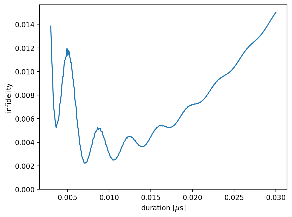
At short pulse durations, the infidelity is high due to leakage out of the computational subspace. At longer durations—corresponding to weaker amplitude—frequency-averaged driving cannot achieve resonance regardless of the nuclear spin state, leading to a gradual increase in infidelity. Bloch–Siegert oscillations appear due to the presence of the counter-rotating term, which is retained since the rotating wave approximation (RWA) is not applied.

To observe the leakage explicitly, we can calculate it as follows:

def leakage(duration, model):

    period_time = 4 * duration
    amplitude = model.rabi_cycle_amplitude_qubit(driving_field_name = 'MW_x',
                                                 spin_name = 'e', 
                                                 period_time = period_time)
    
    model.remove_all_pulses()
    model.driving_field('MW_x').add_rectangle_pulse(frequency = frequency,
                                                    amplitude = amplitude,
                                                    duration = duration,
                                                    phase = 0)

    result = model.simulate_time_evolution(n_eval=2)
    return result.leakage()

leakages = np.array([leakage(duration, model) for duration in durations])

plt.plot(durations, leakages, '-')
plt.xlabel('duration [$\mu$s]')
plt.ylabel('leakage')
plt.ylim(0)
plt.show()

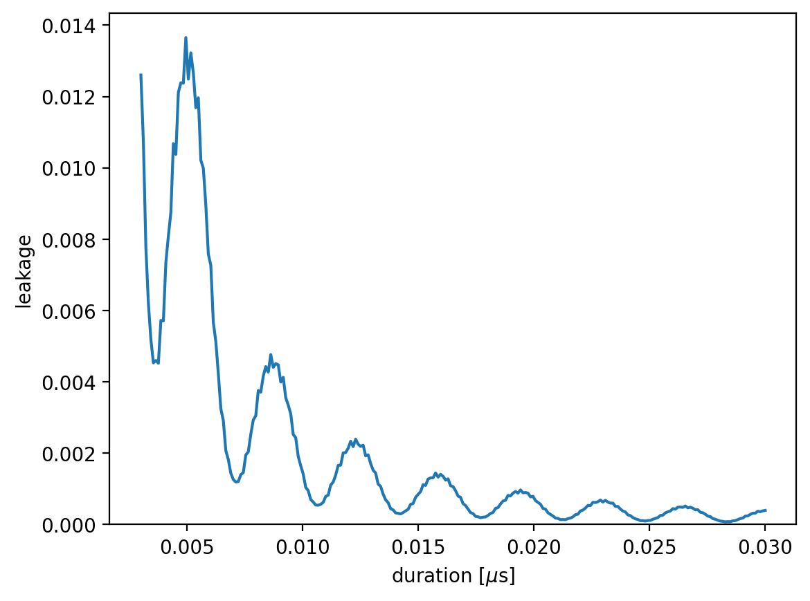
The optimal pulse duration is:

durations[np.argmin(infidelities)]

np.float64(0.007104)

Autodiff with JAX and Simple Gradient Descent

To compute the gradient, we use JAX’s value_and_grad function:

from jax import value_and_grad

value_and_grad_infidelity = value_and_grad(infidelity)

The value_and_grad_infidelity function works similarly to the infidelity function, but returns a tuple:

• The first element is the infidelity value.

• The second element is the gradient with respect to the first argument of the infidelity function, returned as a JAX Array:

duration = 0.03
value_and_grad_infidelity(duration, model)

(Array(0.0150144, dtype=float64),
 Array(1.3289286, dtype=float64, weak_type=True))

We illustrate gate optimization starting from an initial pulse duration using gradient descent. The procedure involves iteratively computing the gradient and updating the duration according to:

\[ \text{duration}_{i+1} = \text{duration}_{i} - \epsilon \cdot \text{grad}_i, \]

where \(\epsilon\) is the learning rate:

duration = 0.03
epsilon = 1e-3
n_step = 25

infidelities_optimized = []
durations_optimized = []

for i in range(n_step):
    
    value, grad = value_and_grad_infidelity(duration, model)
    infidelities_optimized.append(value)
    durations_optimized.append(duration)

    duration -= epsilon*grad
    print(f'{i+1}/{n_step}', end=' ')

1/25 2/25 3/25 4/25 5/25 6/25 7/25 8/25 9/25 10/25 11/25 12/25 13/25 14/25 15/25 16/25 17/25 18/25 19/25 20/25 21/25 22/25 23/25 24/25 25/25 

We can visualize the optimization process:

fig, axs = plt.subplots(1, 2, figsize=(12,4))

axs[0].plot(infidelities_optimized, 'o-', c='#ff7f0e')
axs[0].set_xlabel('steps')
axs[0].set_ylabel('infidelity')
axs[0].set_ylim(0)

axs[1].plot(durations, infidelities, '-')
axs[1].plot(durations_optimized, infidelities_optimized, '.-')
axs[1].set_xlabel('duration [$\mu$s]')
axs[1].set_ylabel('infidelity')
axs[1].set_ylim(0)

plt.show()

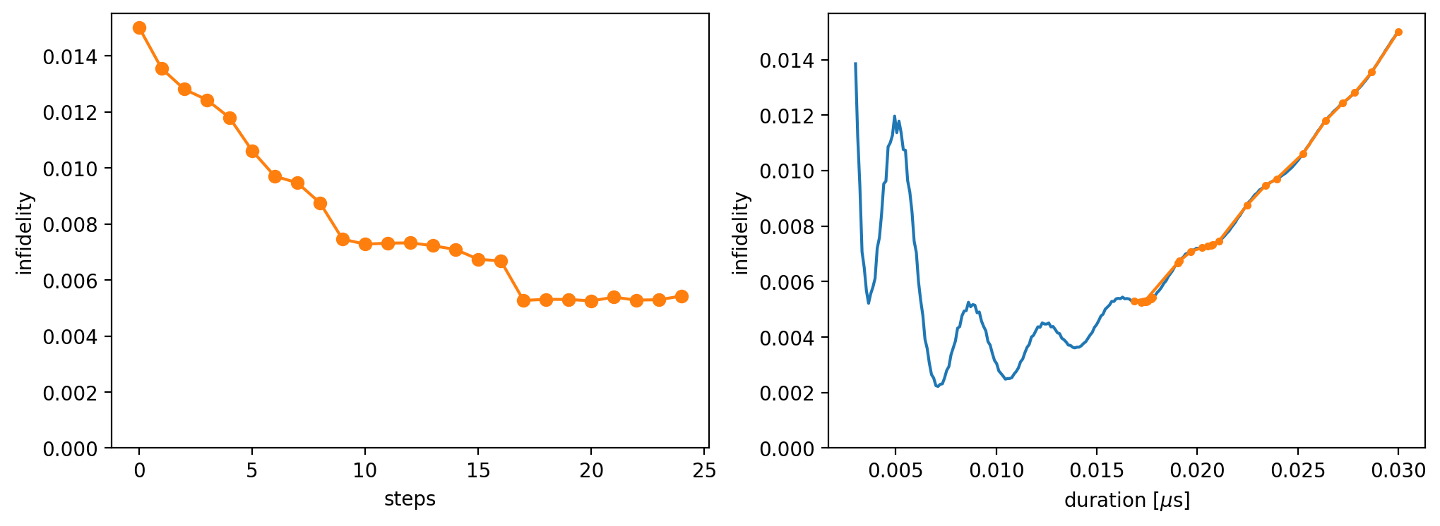
In the left plot, the infidelity is shown as a function of the number of optimization steps. In the right plot, we show the trajectory of the optimization on the landscape.

Note: For oscillatory landscapes, the optimization problem becomes non-trivial and may require a more sophisticated optimization method.

Optimize a Pulse Sequence

As a second example, we consider a more complex scenario: optimizing a pulse sequence with a piecewise-constant envelope. The optimization variables are real numbers, where:

• even-indexed parameters correspond to the real parts of the envelope segments

• odd-indexed parameters correspond to the imaginary parts

def infidelity_2(parameters, dt, model):

    samples = parameters[::2] + 1j*parameters[1::2]
    
    model.remove_all_pulses()
    model.driving_field('MW_x').add_discrete_pulse(frequency = frequency,
                                                   samples = samples,
                                                   dt = dt)

    result = model.simulate_time_evolution(n_eval=2)
    result.ideal = qc
    return 1 - result.average_gate_fidelity()

value_and_grad_infidelity_2 = value_and_grad(infidelity_2)

Gradient descent is initialized from a randomly generated pulse sequence. The sequence consists of 8 constant-envelope pulse segments with a total duration of 0.01 μs. The optimization runs for 100 iterations.

Note: Executing this code may take several minutes, depending on system performance:

np.random.seed(42)

N = 8
duration = 0.01
dt = duration / N
parameters = 0.1 * (np.random.random(2 * N) - 0.5)

epsilon = 2e-5
n_step = 100

infidelities_optimized = []

for i in range(n_step):
    
    value, grads = value_and_grad_infidelity_2(parameters, dt, model)
    infidelities_optimized.append(value)

    parameters -= epsilon*grads
    print(f'{i+1}/{n_step}', end=' ')

1/100 2/100 3/100 4/100 5/100 6/100 7/100 8/100 9/100 10/100 11/100 12/100 13/100 14/100 15/100 16/100 17/100 18/100 19/100 20/100 21/100 22/100 23/100 24/100 25/100 26/100 27/100 28/100 29/100 30/100 31/100 32/100 33/100 34/100 35/100 36/100 37/100 38/100 39/100 40/100 41/100 42/100 43/100 44/100 45/100 46/100 47/100 48/100 49/100 50/100 51/100 52/100 53/100 54/100 55/100 56/100 57/100 58/100 59/100 60/100 61/100 62/100 63/100 64/100 65/100 66/100 67/100 68/100 69/100 70/100 71/100 72/100 73/100 74/100 75/100 76/100 77/100 78/100 79/100 80/100 81/100 82/100 83/100 84/100 85/100 86/100 87/100 88/100 89/100 90/100 91/100 92/100 93/100 94/100 95/100 96/100 97/100 98/100 99/100 100/100 

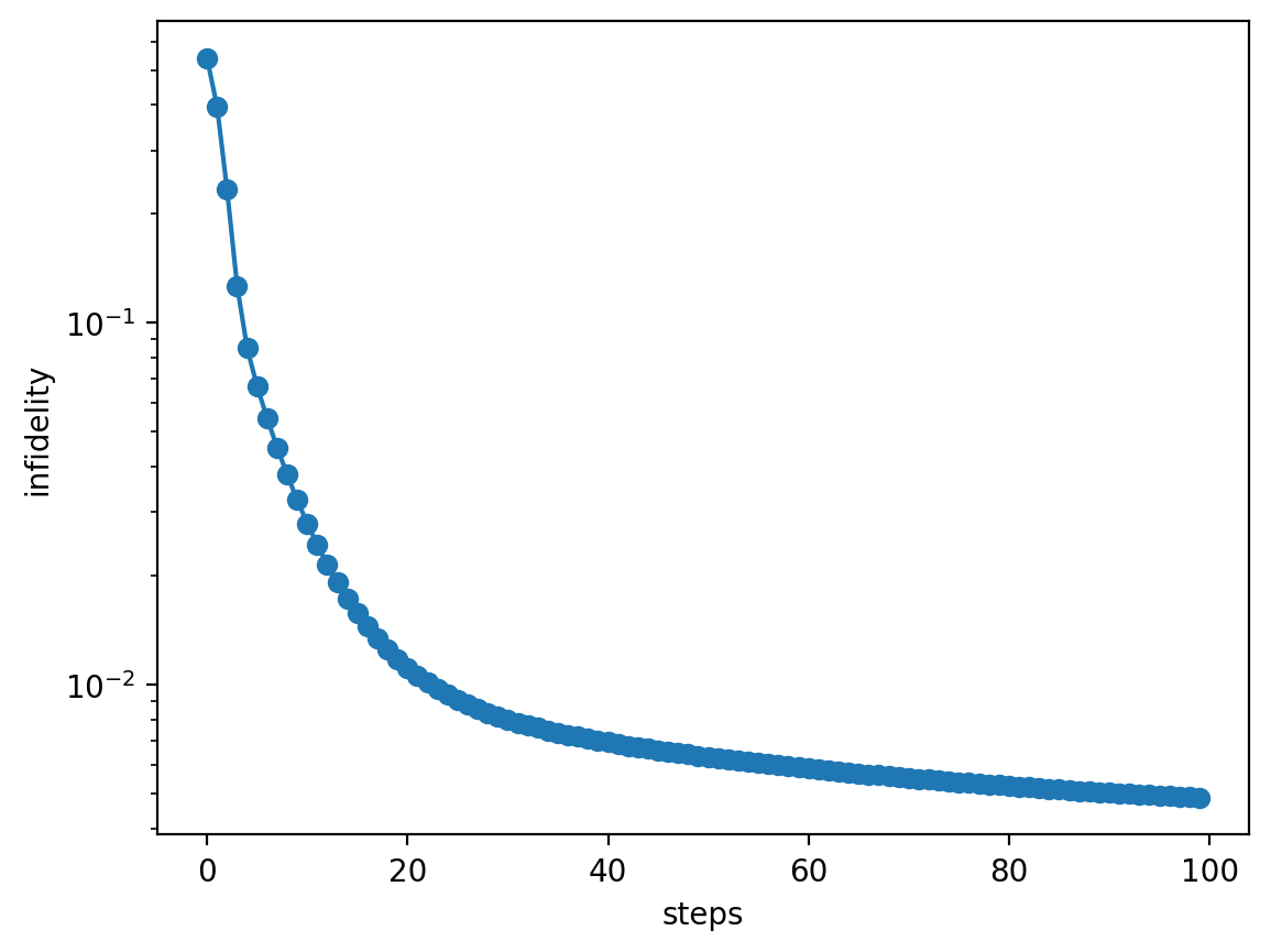
Infidelity is plotted as a function of the number of optimization steps. Starting from an initial gate with infidelity near unity, the optimization gradually converges toward zero infidelity using a highly conservative learning rate.

While a higher learning rate could accelerate convergence, it often leads to suboptimal gate performance. In such cases, more advanced optimization methods are needed to achieve better gate fidelities and faster convergence.

plt.plot(infidelities_optimized, 'o-')
plt.ylabel('infidelity')
plt.xlabel('steps')
plt.yscale('log')
plt.show()

The resulting optimized pulse sequence is shown below:

model.driving_field('MW_x').plot_pulses(function='complex_envelope')

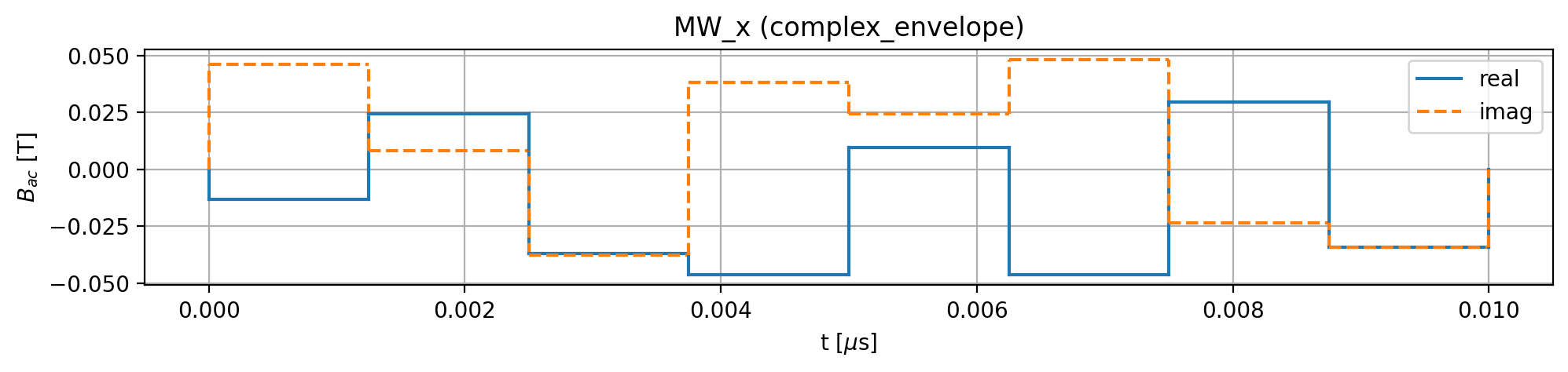
Note: This optimization process is conceptually similar to the Gradient Ascent Pulse Engineering (GRAPE) method, but does not rely on the rotating wave approximation (RWA).