Default nitrogen-vacancy model and multiqubit tutorial

Simphony is a Python package designed for simulating the spin dynamics of point defects, particularly the nitrogen-vacancy (NV) center, which is surrounded by nuclear spins and utilized as a central-spin quantum register.

The main goal of this tutorial is to introduce the predefined NV center model and demonstrate Simphony’s multiqubit capabilities. We illustrate this by simulating a phase gate acting on three nuclear spins, with the electron spin serving as an ancilla.

Import the packages

We import Simphony using the CPU as the default backend:

import numpy as np

import simphony
simphony.Config.set_matplotlib_format('retina')

from qiskit import QuantumCircuit
from qiskit.circuit.library import RXGate

Default NV model

Simphony provides a built-in function to construct a default NV center model. Using the default_nv_model() function, you can define a model containing a single NV electron spin. A nitrogen nuclear spin can be added by specifying its isotope number through the nitrogen_isotope argument, which must be 14, 15, or None. Additional carbon-13 nuclear spins can be included using the carbon_atom_indices argument, which must be a list of tuples.

Each tuple \((n_1, n_2, n_3, n_4)\) defines the position of a carbon atom as:

\[ \text{carbon atom position} = n_1 \cdot \mathbf{a}_1 + n_2 \cdot \mathbf{a}_2 + n_3 \cdot \mathbf{a}_3 + n_4 \cdot \boldsymbol{\tau}, \]

where \(\mathbf{a}_1\), \(\mathbf{a}_2\), and \(\mathbf{a}_3\) are the primitive lattice vectors, and \(\mathbf{0}\) and \(\boldsymbol{\tau}\) are the positions of the carbon atoms inside the primitive cell. The indices \(n_1\), \(n_2\), \(n_3\) are integers, and \(n_4\) is either \(0\) or \(1\). Our convention is:

\[\begin{split} \begin{aligned} \mathbf{a}_1 &= a_\text{CC}\cdot \left( 0, \frac{2\sqrt{2}}{3}, \frac{4}{3} \right), \\ \mathbf{a}_2 &= a_\text{CC}\cdot \left( -\frac{\sqrt{6}}{3}, -\frac{\sqrt{2}}{3}, \frac{4}{3} \right), \\ \mathbf{a}_3 &= a_\text{CC}\cdot \left( \frac{\sqrt{6}}{3}, -\frac{\sqrt{2}}{3}, \frac{4}{3} \right), \\ \boldsymbol{\tau} &= \frac{\mathbf{a}_1 + \mathbf{a}_2 + \mathbf{a}_3}{4} = a_\text{CC}\cdot (0, 0, 1), \end{aligned} \end{split}\]

where \(a_\text{CC} = 0.1545\ \text{nm}\) is the carbon–carbon distance. The nitrogen occupies the \(\boldsymbol{\tau}\) position, while the missing carbon atom (vacancy) corresponds to the \(\mathbf{0}\) lattice point.

A simple spin system consisting of an NV electron spin, a \(^{14}\text{N}\) nuclear spin, and two \(^{13}\text{C}\) nuclear spins can be defined as:

model = simphony.default_nv_model(nitrogen_isotope=14,
                                  static_field_strength=0.05,
                                  carbon_atom_indices=[(1,1,1,0), (2,-3,4,1)],
                                  electron_spin_state='0',
                                  nuclear_spin_state='1')
model.plot_levels()

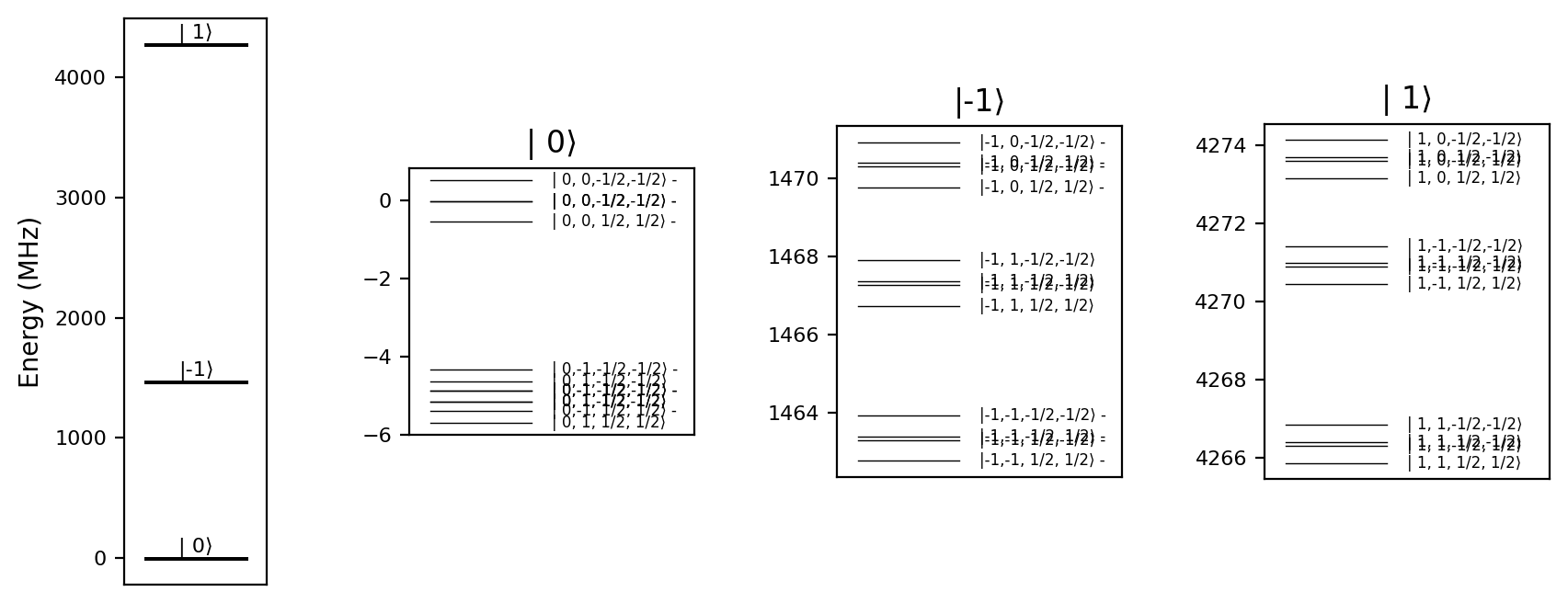
The rotating frame is defined as follows:

• The rotating frame frequency of the electron spin is set to its qubit splitting (transition frequency), conditioned on the nuclear spins being in state \(\ket{1}\).

• The rotating frame frequencies of all nuclear spins are set to their respective qubit splittings, assuming the electron spin is in state \(\ket{0}\) and the other nuclear spins are in state \(\ket{1}\).

The spins included in the model are:

model.spins

[Spin(dimension=3, name='e', qubit_subspace=(0, -1), gyromagnetic_ratio=28020.4, zero_field_splitting=2873.668, local_quasistatic_noise=[0, 0, 0]),
 Spin(dimension=3, name='N', qubit_subspace=(0, -1), gyromagnetic_ratio=-3.077, zero_field_splitting=-4.949156, local_quasistatic_noise=[0, 0, 0]),
 Spin(dimension=2, name='C1', qubit_subspace=(-0.5, 0.5), gyromagnetic_ratio=10.71, zero_field_splitting=0.0, local_quasistatic_noise=[0, 0, 0]),
 Spin(dimension=2, name='C2', qubit_subspace=(-0.5, 0.5), gyromagnetic_ratio=10.71, zero_field_splitting=0.0, local_quasistatic_noise=[0, 0, 0])]

By default, the hyperfine interactions between the electron spin and the nuclear spins are taken from the hyperfine dataset provided by Viktor Ivády’s group:

model.interactions

[Interaction(spin_name_1='e', spin_name_2='N', tensor=[[2.679, 0, 0], [0, 2.679, 0], [0, 0, 2.188218]]),
 Interaction(spin_name_1='e', spin_name_2='C1', tensor=[[-0.067270283415, 3.70794550132416e-07, -7.27906701892158e-08], [3.70794550132416e-07, -0.0672701293583333, -7.09176246990739e-07], [-7.27906701892158e-08, -7.09176246990739e-07, 0.0958844127833333]]),
 Interaction(spin_name_1='e', spin_name_2='C2', tensor=[[0.0050591293382, 0.0038067421256854, 0.0154034100176021], [0.0038067421256854, -0.0096116264187333, 0.003696458093473], [0.0154034100176021, 0.003696458093473, 0.0045524970785333]])]

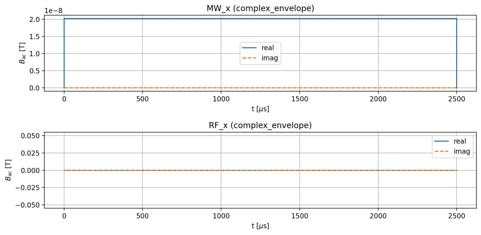
By default, a microwave (MW) and a radio-fequency (RF) field are added to the model. Both driving fields point to the x-direction:

model.driving_fields

[DrivingField(name='MW_x', direction=[1. 0. 0.]),
 DrivingField(name='RF_x', direction=[1. 0. 0.])]

Phase gate

The phase gate is implemented using a weak electron spin resonance (ESR) pulse. This pulse rotates the electron spin by \(2\pi\) if and only if the nuclear spins are in their qubit state \(\ket{1}\). The pulse frequency must match the electron spin splitting when all nuclear spins are in state \(\ket{1}\), which corresponds to the quantum number -1 for the nitrogen and 1/2 for the carbon nuclear spins:

duration = 2500
frequency = model.splitting_qubit('e', rest_quantum_nums={'N': -1, 'C1': 1/2, 'C2': 1/2})
phase = 0
angle = 2 * np.pi
period_time = 2 * np.pi / angle * duration
amplitude = model.rabi_cycle_amplitude_qubit(driving_field_name='MW_x',
                                             period_time=period_time,
                                             spin_name='e',
                                             rest_quantum_nums={'N': -1, 'C1': 1/2, 'C2': 1/2})

model.remove_all_pulses()
model.driving_field('MW_x').add_rectangle_pulse(amplitude=amplitude,
                                                frequency=frequency,
                                                phase=phase,
                                                duration=duration)


model.plot_driving_fields(function='complex_envelope')

Run the simulation for the defined pulse:

result = model.simulate_time_evolution(verbose=True)

start = 0.0
end = 2500.0
solver_method = jax_expm
number of simulated driving terms = 1
number of simulated noise terms = 0
---------------------------------------------------------------------------
simulate time segment [0, 2500] with step size 2.712e-06 (type: single_sine_wave)

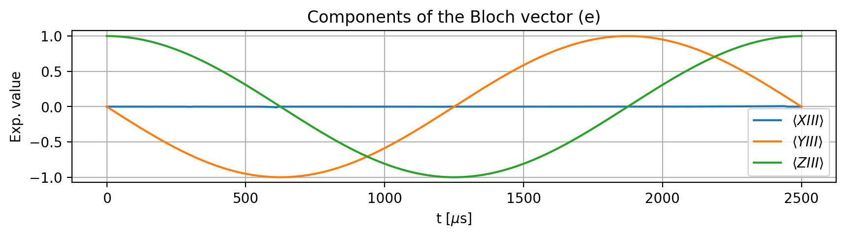
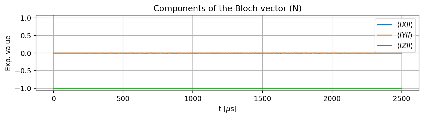
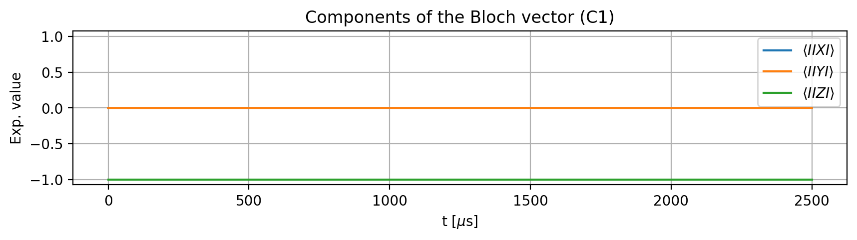
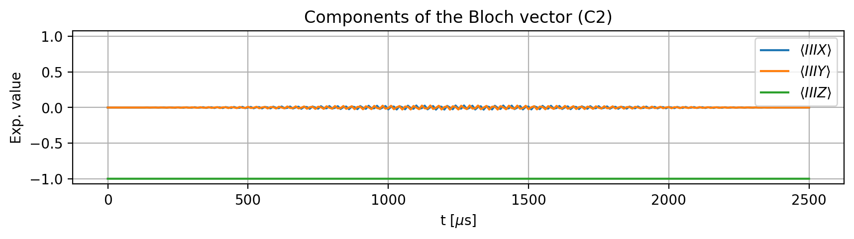
To examine the effect of the pulse, we define an initial state. The electron spin undergoes a \(2\pi\) rotation only when the nuclear spins are in their qubit state \(\ket{1}\), which corresponds to the quantum number -1 for the nitrogen and 1/2 for the carbon nuclear spins. If we change -1 to 0 for N, or 1/2 to -1/2 for either C1 or C2, the rotation should no longer occur:

result.initial_state = model.productstate({'e': 0, 'N': -1, 'C1': 1/2, 'C2': 1/2})
result.plot_Bloch_vectors()

The implemented operation corresponds to a conditional \(\text{RX}(2\pi)\) gate:

qc = QuantumCircuit(4)
qc.append(RXGate(angle).control(3, ctrl_state='111'), [1, 2, 3, 0])
qc.draw()

     ┌────────┐
q_0: ┤ Rx(2π) ├
     └───┬────┘
q_1: ────■─────
         │     
q_2: ────■─────
         │     
q_3: ────■─────
               

The average gate fidelity over the qubit subspace of all spins is:

result.ideal = qc
result.average_gate_fidelity()

np.float64(0.2890966405507237)

If we calculate the average gate fidelity over the nuclear spin subspace only, treating the electron as an ancilla fixed in the state \(\ket{0}\), we obtain:

result.average_gate_fidelity(ancilla_state={'e': '0'})

np.float64(0.997710456231699)

References:

[1] Felton et al., Phys. Rev. B 79, 075203 (2009)
[2] CRC Handbook of Chemistry and Physics, sec. 11-4 (97th edition)