AC magnetometry with an NV center
Simphony is a Python package designed for simulating the spin dynamics of point defects, in particular the nitrogen-vacancy (NV) center, which is surrounded by nuclear spins and serves as a central-spin quantum register.
NV centers are widely used to detect oscillating magnetic fields, since they combine atomic-scale spatial resolution with high sensitivity. In this example notebook we simulate such a measurement from end to end: the electron spin is driven by dynamical decoupling sequences, it accumulates phase from an external AC field during the free-evolution intervals, and the resulting population difference is read out.
We will:
derive the phase accumulated by the electron spin during a pulse sequence
implement a Hahn echo and locate the AC resonance by scanning the free-evolution time
extend the measurement to CPMG sequences with \(n = 2, 3, 6, 10\) \(\pi\)-pulses
measure the spectral resolution and confirm that it improves as \(1/n\)
Phase accumulation during a pulse sequence
In the absence of the AC field, the NV electron spin Hamiltonian (zero-field splitting plus static Zeeman term) is diagonal in the \(S_z\) basis, with eigenstates \(|m_s\rangle\) (\(m_s = 0, \pm 1\)). An oscillating field \(B(t)\) applied along the NV axis adds the perturbation
which is diagonal in the same basis and therefore commutes with the unperturbed Hamiltonian at every instant.
Because \(H_{\text{AC}}(t)\) commutes with \(H_0\), it cannot drive transitions between the \(m_s\) levels. Provided it also varies slowly compared with the other NV transition frequencies, the adiabatic theorem guarantees that the spin remains in whichever instantaneous eigenstate it started in, picking up an extra dynamical phase
The factor of \(2\pi\) appears because Simphony works in \(\hbar = 1/2\pi\) units. For a superposition of the two qubit sublevels (\(m_s = 0\) and \(m_s = -1\) in the default Simphony NV model), the relative phase between the two branches accumulates as
A resonant \(\pi\)-pulse swaps the populations and coherences of the two qubit levels, which is equivalent to reversing the sign of \(m_s\) for the remainder of the sequence. The phase accumulated during each subsequent free-evolution interval therefore enters with the opposite sign. Summing over all intervals between \(m\) pulses applied at times \(t_1 < t_2 < \cdots < t_m\) gives the alternating-sign structure
which is the formula used throughout this notebook.
The derivation assumes the AC field varies slowly compared with the gaps to states outside the qubit subspace, i.e. \(f_{\text{AC}} \ll D,\, \gamma_e B_0\). This is comfortably satisfied for the kHz–MHz signals that AC magnetometry targets.
Reference. B. Naydenov, F. Dolde, L. T. Hall, C. Shin, H. Fedder, L. C. L. Hollenberg, F. Jelezko, and J. Wrachtrup, Dynamical decoupling of a single-electron spin at room temperature, Phys. Rev. B 83, 081201(R) (2011).
Dynamical decoupling sequences
For an oscillating field \(B(t) = B_{\text{AC}} \cos(2\pi f_{\text{AC}} t + \varphi)\), the phase accumulated by the spin depends on how the \(\pi\)-pulses are placed relative to the field oscillation. The two most common sequences are:
Hahn echo: \(\frac{\pi}{2}_x - \tau - \pi_x - \tau - \frac{\pi}{2}_x\)
Carr–Purcell–Meiboom–Gill (CPMG): \(\frac{\pi}{2}_x - (\tau - \pi_y - \tau)^n - \frac{\pi}{2}_x\)
where the subscripts denote the rotation axes. The accumulated phase \(\Delta \Phi\) is maximal when the pulse spacing is resonant with the AC period: \(f_{\text{AC}} = 1/(2\tau)\) for the Hahn echo and \(f_{\text{AC}} = 1/(4\tau)\) for CPMG, since there the pulse spacing is \(2\tau\). On resonance the AC field contributes constructively during every free-evolution interval, while static noise is refocused by the \(\pi\)-pulses.
Optical readout
The accumulated phase is not observed directly; it is converted into a population difference. The \(m_s = 0\) sublevel decays back to the orbital ground state largely through spin-conserving fluorescence, whereas the \(m_s = \pm 1\) sublevels have a significant branching ratio into a metastable singlet via a spin-selective intersystem crossing. That path is dark, so population in \(m_s = \pm 1\) appears as reduced photoluminescence.
After the final \(\pi/2\)-pulse the population difference between the two qubit levels is mapped onto the accumulated phase as
a Ramsey-type interferometric readout. This is exactly the quantity returned by
expectation_value('ZI', ...) in the simulations below.
Import the packages
Import the required packages and set the computation to run on the GPU:
import numpy as np
np.set_printoptions(linewidth=200, precision=4) # to print wide matrices

import simphony
simphony.Config.set_platform('gpu')
simphony.Config.set_matplotlib_format('retina')
from jax import value_and_grad
from qiskit import QuantumCircuit
from matplotlib import pyplot as plt
from scipy.optimize import minimize
from scipy.stats import norm
plt.rcParams.update({'font.size': 14})
Pulse and field parameters
The whole notebook is driven by three constants, so the measurement can be moved to a different operating point by editing a single cell. Both pulse durations are chosen much shorter than the AC period, so that the pulses are close to instantaneous on the timescale of the phase accumulation:
# Rectangular MW pulse durations. Both are far shorter than the AC period, so the pulses are
# near-instantaneous on the timescale of the phase accumulation.
duration1, duration2 = 0.01, 0.02      # pi/2 and pi pulse durations [us]

# Static field along the NV axis. It sets the separation between the two electron spin
# transitions, and therefore how selectively a strong MW pulse addresses the qubit one.
B0 = 0.0045                            # [T]

print(f'pi/2 pulse: {duration1} us  ->  Rabi frequency {1 / (4 * duration1):.1f} MHz')
print(f'pi   pulse: {duration2} us  ->  Rabi frequency {1 / (2 * duration2):.1f} MHz')
print(f'static field B0 = {B0 * 1e3:.2f} mT')
pi/2 pulse: 0.01 us  ->  Rabi frequency 25.0 MHz
pi   pulse: 0.02 us  ->  Rabi frequency 25.0 MHz
static field B0 = 4.50 mT
Hahn echo
The Hahn echo is the simplest dynamical decoupling sequence for AC magnetometry:
the electron spin is initialized in \(|0\rangle\)
a \(\pi/2\)-pulse prepares the superposition \(\frac{1}{\sqrt{2}}(|0\rangle + |1\rangle)\)
the spin evolves freely for a time \(\tau\) in the presence of the AC field
a \(\pi\)-pulse inverts the qubit levels, flipping the sign of the accumulated phase
a second free-evolution interval of duration \(\tau\) follows
a final \(\pi/2\)-pulse converts the accumulated phase into a population difference
The total sequence time is \(T = 2\tau + t_{\pi/2} + t_{\pi}\). Since \(t_{\pi/2}, t_{\pi} \ll \tau\), the resonance appears where \(f_{\text{AC}} \approx 1/(2\tau)\): the phase contributions from the two intervals then add constructively. Static field noise, being constant over the sequence, is cancelled by the \(\pi\)-pulse.
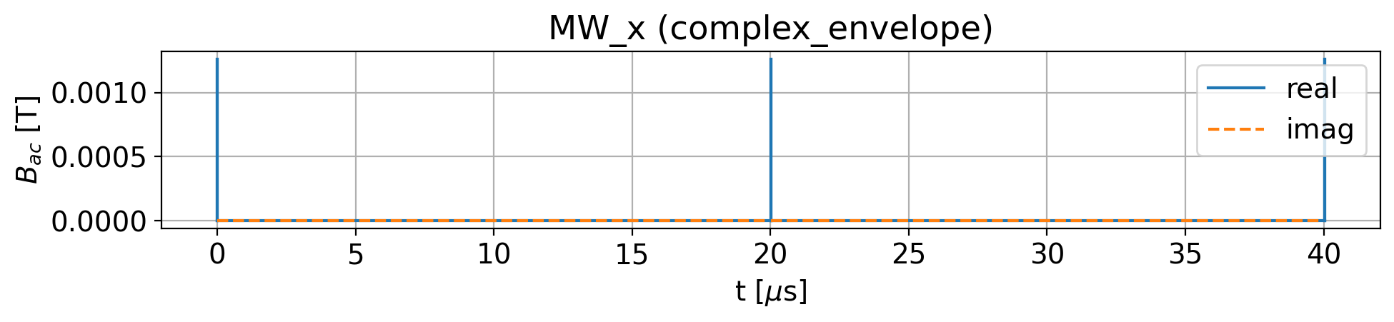
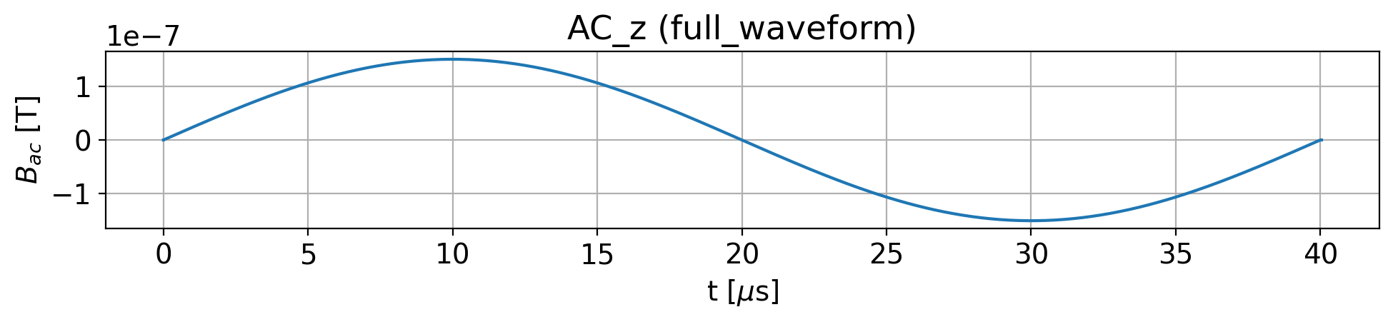
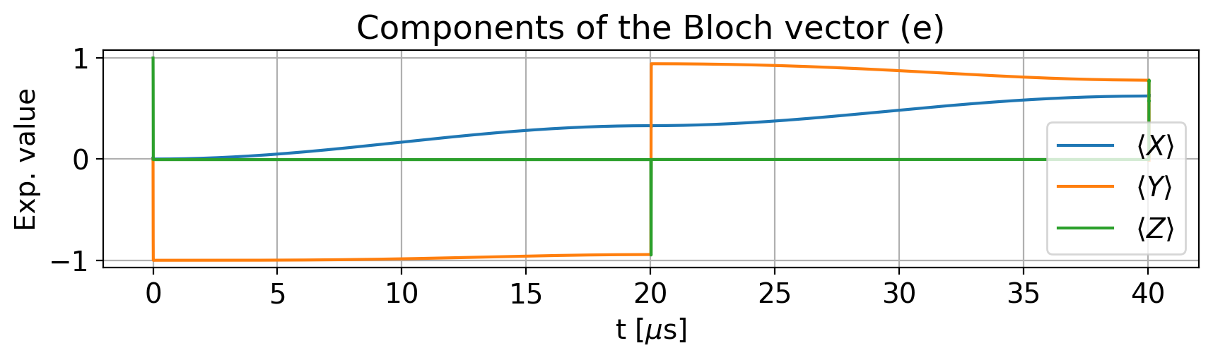
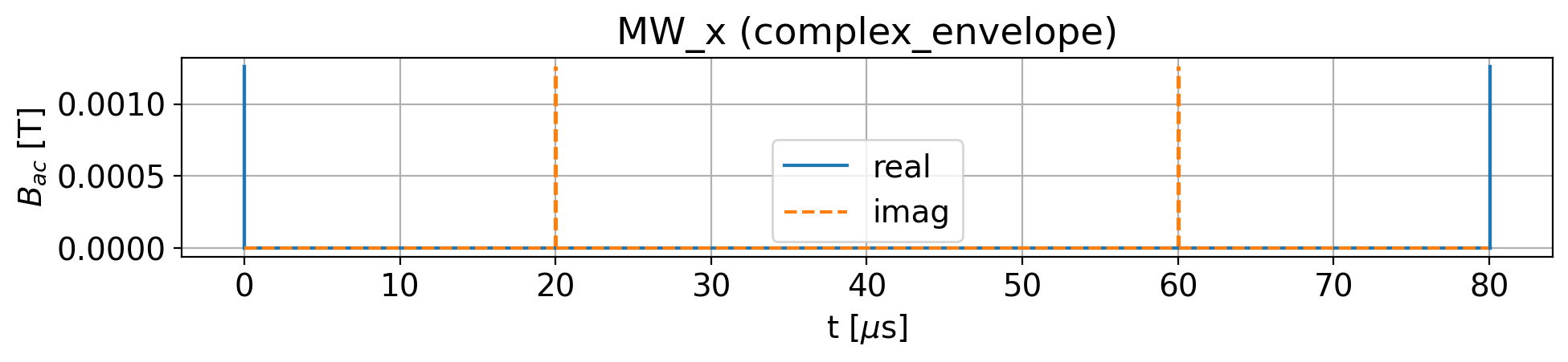
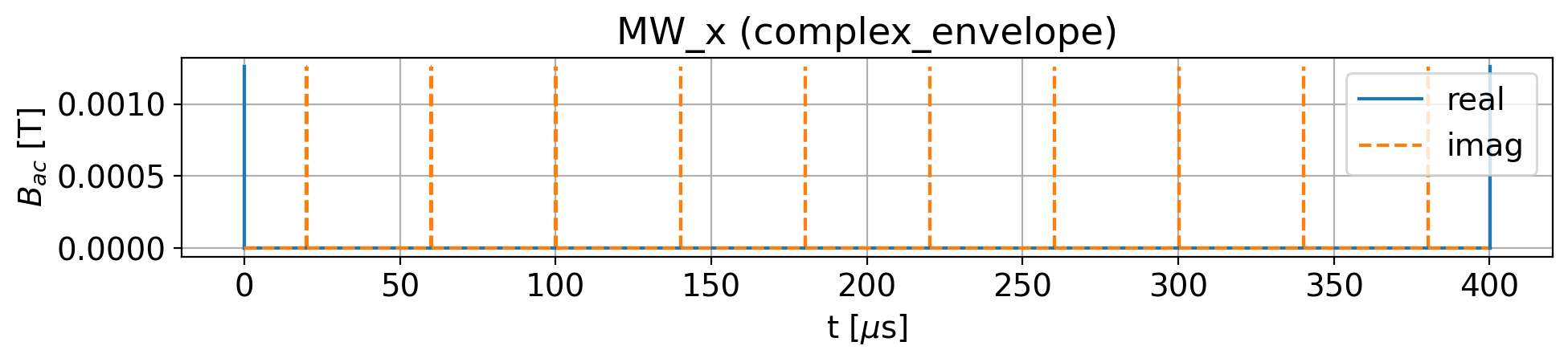
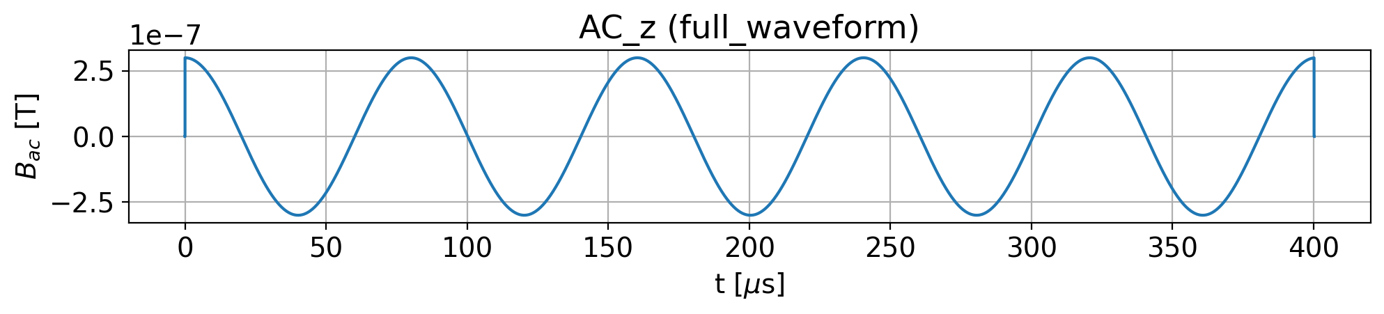
First, we build one sequence explicitly and inspect it. The cell below plots the
MW envelope and the AC waveform, and follows the electron spin on the Bloch sphere.
Setting b_AC = 0.0 is a useful sanity check: without the AC field the echo returns the spin to its
starting point and no net phase accumulates:
# Demonstration of the accumulated phase difference
model_no_n = simphony.default_nv_model(nitrogen_isotope=None,
                                  static_field_strength=0.05)
driving_field_AC = simphony.LinearDrivingField(direction = [0, 0, 1], name = 'AC_z') #the measured AC field in the z direction
model_no_n.add_driving_field(driving_field_AC)

t_period = 20.
f_ac_mhz = 1/ (2*t_period)

tau = 20. #resonant case
#tau = 23. #offresonant case
freq_pulse = model_no_n.splitting_qubit('e')      # frequency of the pulses

#b_AC = 0.0  #no external AC field, no accumulating phase
b_AC = 0.00000015
print('Larmor frequency (MHz): ', freq_pulse)
print('AC frequency (MHz): ', f_ac_mhz)

amplitude_half_pi = model_no_n.rabi_amplitude_qubit(
                        driving_field_name='MW_x',
                        period_time = 2 * np.pi * duration1 / (np.pi / 2),
                        spin_name='e')
amplitude_pi = model_no_n.rabi_amplitude_qubit(
                        driving_field_name='MW_x',
                        period_time = 2 * np.pi * duration2 / (np.pi ),
                        spin_name='e')

model_no_n.remove_all_pulses()
model_no_n.driving_field('AC_z').add_wait(duration1)
model_no_n.driving_field('AC_z').add_rectangle_pulse(
                        amplitude=b_AC,
                        frequency=f_ac_mhz,
                        phase=-np.pi/2,
                        duration=2 * tau,
                        start = duration1)

model_no_n.driving_field('MW_x').add_rectangle_pulse(
                        amplitude=amplitude_half_pi,
                        frequency=freq_pulse,
                        phase=0,
                        duration=duration1)
model_no_n.driving_field('MW_x').add_wait(tau)
model_no_n.driving_field('MW_x').add_rectangle_pulse(
                        amplitude=amplitude_pi,
                        frequency=freq_pulse,
                        phase=0,
                        duration=duration2)
model_no_n.driving_field('MW_x').add_wait(tau)
model_no_n.driving_field('MW_x').add_rectangle_pulse(
                        amplitude=amplitude_half_pi,
                        frequency=freq_pulse,
                        phase=0,
                        duration=duration1)

model_no_n.plot_driving_fields(name = 'MW_x', function='complex_envelope')
model_no_n.plot_driving_fields(name = 'AC_z', function='full_waveform')
result = model_no_n.simulate_time_evolution(apply_noise=False)
result.initial_state = model_no_n.productstate({'e': 0})
result.plot_Bloch_vectors(frame='rotating')
Larmor frequency (MHz):  1470.3450000000003
AC frequency (MHz):  0.025
Scanning the free-evolution time
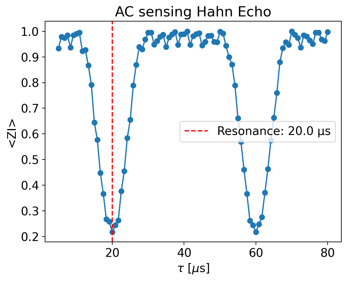
Next we wrap the sequence into a function that returns \(\langle ZI \rangle\), and scan \(\tau\) to locate the resonance:
# Full wrapped function to simulate the electronic <Z> expectation value
def Hahn_echo(model, wait, f_ac_mhz, B_ac_tesla, apply_noise=False, n_shots=1, ac_phase=np.pi/2):


    frequency = model.splitting_qubit('e', rest_quantum_nums={'N': 0})

    angle1 = np.pi / 2
    period_time1 = 2 * np.pi * duration1 / angle1
    angle2 = np.pi
    period_time2 = 2 * np.pi * duration2 / angle2

    amplitude1 = model.rabi_cycle_amplitude_qubit(
        driving_field_name='MW_x',
        period_time=period_time1,
        spin_name='e'
    )
    amplitude2 = model.rabi_cycle_amplitude_qubit(
        driving_field_name='MW_x',
        period_time=period_time2,
        spin_name='e'
    )

    model.remove_all_pulses()
    model.driving_field('AC_z').add_wait(duration1)
    model.driving_field('AC_z').add_rectangle_pulse(amplitude=B_ac_tesla,
                                                            frequency=f_ac_mhz,
                                                            phase=ac_phase,
                                                            duration=2*wait+duration2)
    model.driving_field('MW_x').add_rectangle_pulse(
        amplitude=amplitude1,
        frequency=frequency,
        phase=0,
        duration=duration1
    )

    model.driving_field('MW_x').add_wait(wait)
    model.driving_field('MW_x').add_rectangle_pulse(
        amplitude=amplitude2,
        frequency=frequency,
        phase=0,
        duration=duration2
    )

    model.driving_field('MW_x').add_wait(wait)
    model.driving_field('MW_x').add_rectangle_pulse(
        amplitude=amplitude1,
        frequency=frequency,
        phase=0,
        duration=duration1
    )
    result = model.simulate_time_evolution(n_eval=2, apply_noise=apply_noise, n_shots=n_shots)
    result.initial_state = model.productstate({'e': 0,'N':0})
    expectation_value = result.expectation_value('ZI', t_idx=-1, shot='all', frame='rotating')

    return expectation_value[:, 0, 0]
t_period = 20
frequency_target = 1/(t_period*2)
B_ac =  3e-7
tau_values = np.linspace(5,80,91)

signals_hahn = np.zeros(tau_values.shape[0])
for idx,tau in enumerate(tau_values):
    model = simphony.default_nv_model(nitrogen_isotope=14, static_field_strength=B0)
    outside_field = simphony.LinearDrivingField(
        direction=[0, 0, 1],
        name="AC_z"
    )
    model.add_driving_field(outside_field)
    signals_hahn[idx] = Hahn_echo(model, tau, f_ac_mhz=frequency_target, B_ac_tesla=B_ac,
                             apply_noise=False, n_shots=1)[0]
plt.plot(tau_values, signals_hahn, 'o-')
plt.axvline(t_period, color='r', linestyle='--', label=f'Resonance: {t_period:.1f} µs')
plt.legend()
plt.xlabel(r"$\tau$ [$\mu$s]")
plt.ylabel("<ZI>")
plt.title("AC sensing Hahn Echo")
plt.show()
Comparison with the analytic filter function
For an ideal sequence of instantaneous pulses, the accumulated phase can be written in closed form:
We take the electron gyromagnetic ratio directly from the model
(model.spin('e').gyromagnetic_ratio, in MHz/T) so that the comparison is self-consistent with the
simulation:
def delta_phi_analytic(gamma_e_mhz_per_t, B_ac_tesla, f_ac_mhz, tau, phi):
    omega = 2 * np.pi * f_ac_mhz
    return gamma_e_mhz_per_t * B_ac_tesla / f_ac_mhz * (
        2 * np.sin(omega * tau + phi) - np.sin(2 * omega * tau + phi) - np.sin(phi)
    )

gamma_e = model.spin('e').gyromagnetic_ratio  # MHz/T
tau_fine = np.linspace(tau_values[0], tau_values[-1], 400)
analytic_signal = np.cos(delta_phi_analytic(gamma_e, B_ac, frequency_target, tau_fine, np.pi / 2))

fig, ax = plt.subplots()
ax.plot(tau_values, signals_hahn, 'o--', label='simulated')
ax.plot(tau_fine, analytic_signal, '-', label='ideal analytic', alpha=0.7)
ax.axvline(t_period, color='r', linestyle='--', label=f'Resonance: {t_period:.1f} µs')
ax.set_xlabel(r"$\tau$ [$\mu$s]")
ax.set_ylabel(r"$\langle ZI \rangle$ / $\cos(\Delta\Phi)$")
ax.set_title("Simulated vs. ideal analytic Hahn-echo resonance")
ax.legend()
plt.show()
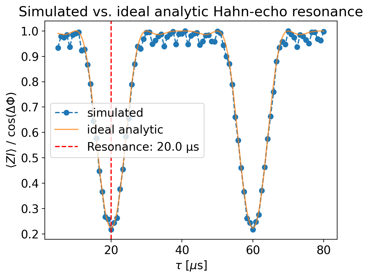
The closed form dips at the same \(\tau = 20, 60, \ldots\,\mu\text{s}\) as the simulation, which confirms the resonance location. The two curves do not match perfectly in amplitude, because the analytic formula assumes instantaneous pulses and a two-level system, while the simulation includes the finite pulse durations and the full multi-level NV Hamiltonian.
The signal falls off smoothly on either side of the resonance. Since \(f_{\text{AC}}\) is held fixed while \(\tau\) is swept, the resonance condition is also met at odd multiples of \(\tau_{\text{res}}\). The width of the central feature is set by the total sensing time: longer sequences give sharper resonances, which is what CPMG exploits.
Phase scan
In practice the phase \(\varphi\) of the AC field is unknown. Measuring the signal over a grid of \(\tau\) and \(\varphi\) values removes the need to know it in advance, because for every \(\tau\) there is some phase that gives a strong response. For a Hahn echo the accumulated phase is
On resonance the two integrals have equal magnitude and opposite sign, giving maximal interference at \(\varphi = \pi/2\):
#running this cell might take a while
tau_res = 20
frequency_target = 1 / (tau_res * 2 + duration2)
B_ac = 3e-7

tau_values_hahn_hm = np.linspace(5, 35, 31) #tau values Hahn heatmap
phase_values = np.linspace(0, 2 * np.pi, 37)

heatmap = np.zeros((len(phase_values), len(tau_values_hahn_hm)))

for i, phase in enumerate(phase_values):
    for j, tau in enumerate(tau_values_hahn_hm):
        model = simphony.default_nv_model(nitrogen_isotope=14, static_field_strength=B0)
        outside_field = simphony.LinearDrivingField(direction=[0, 0, 1], name="AC_z")
        model.add_driving_field(outside_field)
        heatmap[i, j] = Hahn_echo(model, tau, f_ac_mhz=frequency_target, B_ac_tesla=B_ac,
                                   apply_noise=False, n_shots=1, ac_phase=phase)[0]
fig, ax = plt.subplots(figsize=(8, 5))
im = ax.pcolormesh(tau_values_hahn_hm, phase_values, heatmap, cmap='viridis', shading='auto')
fig.colorbar(im, ax=ax, label='<ZI>')
#ax.axvline(tau_res, color='k', linestyle='--', linewidth=1, label=f'Resonance τ = {tau_res} µs') # TODO: decide if to keep this line or not.
ax.set_xlabel(r'$\tau$ [µs]')
ax.set_ylabel(r'AC phase [$\text{rad}$]')
ax.set_yticks(np.arange(0, np.pi*2.1, np.pi*0.5))
ax.set_title('Hahn Echo: phase vs τ heatmap')
plt.tight_layout()
plt.savefig('heatmap_Bac_phase_fixed.pdf')
plt.show()
# Slice at a specific phase value
idx = 18
print(f"Phase value at index {idx}: {phase_values[idx]:.2f} rad")
tau_values = np.linspace(5, 35, 31)
tau_temp = heatmap[idx,:]

gamma_e = model.spin('e').gyromagnetic_ratio  # MHz/T
tau_fine = np.linspace(tau_values[0], tau_values[-1], 400)
analytic_signal = np.cos(delta_phi_analytic(gamma_e, B_ac, frequency_target, tau_fine, phase_values[idx]))


fig, ax = plt.subplots()
ax.plot(tau_values, tau_temp, 'o--', label='simulated')
ax.plot(tau_fine, analytic_signal, '-', label='ideal analytic', alpha=0.7)
#ax.axvline(t_period, color='r', linestyle='--', label=f'Resonance: {t_period:.1f} µs')
ax.set_xlabel(r"$\tau$ [$\mu$s]")
ax.set_ylabel(r"$\langle ZI \rangle$ / $\cos(\Delta\Phi)$")
ax.set_title(f"Slice of the heatmap at AC phase = {phase_values[idx]:.2f} rad")
ax.legend()
plt.show()
Phase value at index 18: 3.14 rad
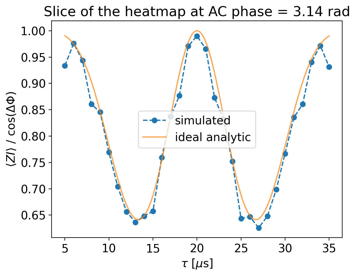
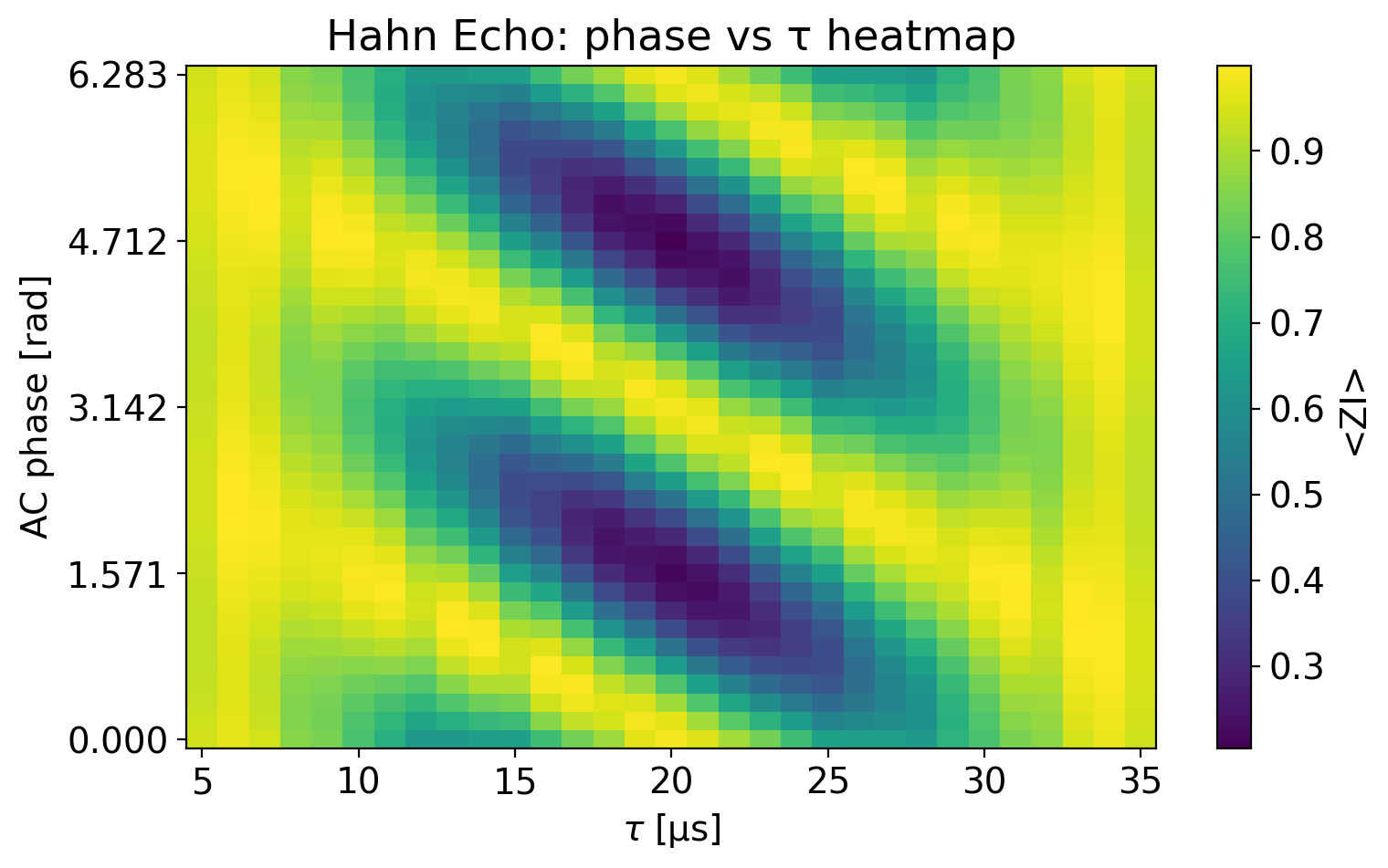
The heatmap shows vertical fringes at the resonance condition \(\tau \approx 20\,\mu\)s, with a sinusoidal variation along the phase axis that reflects the \(\cos(\varphi)\) dependence of the accumulated phase.
The resonance can therefore be identified without prior knowledge of the AC phase, by finding the \(\tau\) that maximizes the signal amplitude across all phases.
CPMG sequences
CPMG extends the Hahn echo by applying several \(\pi\)-pulses during the sensing time:
The total sensing time grows to \(T \approx 2n\tau\), which brings three advantages:
Narrower resonances. The filter function width scales as \(\Delta f \sim 1/T\), so the resonance sharpens as \(1/n\) and the frequency resolution improves.
Better noise suppression. Additional \(\pi\)-pulses refocus low-frequency noise more effectively, extending the coherence time.
A different resonance condition. The spacing between consecutive \(\pi\)-pulses is \(2\tau\), so the resonance sits at \(f_{\text{AC}} = 1/(4\tau)\).
The CPMG function below builds the sequence for an arbitrary number of pulses:
def CPMG(model, wait, f_ac_mhz, B_ac_tesla, apply_noise=False, n_shots=1, n=2,
         plot=False, n_split=250):


    has_nitrogen = 'N' in model.spin_names
    rest_quantum_nums = {'N': 0} if has_nitrogen else None
    initial_state = {'e': 0, 'N': 0} if has_nitrogen else {'e': 0}
    observable = 'ZI' if has_nitrogen else 'Z'

    frequency = model.splitting_qubit('e', rest_quantum_nums=rest_quantum_nums)

    angle1 = np.pi / 2
    period_time1 = 2 * np.pi * duration1 / angle1
    angle2 = np.pi
    period_time2 = 2 * np.pi * duration2 / angle2

    amplitude1 = model.rabi_cycle_amplitude_qubit(
        driving_field_name='MW_x',
        period_time=period_time1,
        spin_name='e'
    )
    amplitude2 = model.rabi_cycle_amplitude_qubit(
        driving_field_name='MW_x',
        period_time=period_time2,
        spin_name='e'
    )

    model.remove_all_pulses()
    model.driving_field('AC_z').add_wait(duration1)
    model.driving_field('AC_z').add_rectangle_pulse(amplitude=B_ac_tesla,
                                                            frequency=f_ac_mhz,
                                                            phase= ( - duration1*2*np.pi*f_ac_mhz), #phase= (np.pi/2 - (duration1+duration2+wait)*2*np.pi*f_ac_mhz),
                                                            duration=2*(n)*wait+(n-2)*duration2)
    model.driving_field('MW_x').add_rectangle_pulse(amplitude=amplitude1,
                                                    frequency=frequency,
                                                    phase=0, #rotating around the x-axis
                                                    duration=duration1)
    for i in range(n):
        model.driving_field('MW_x').add_wait(wait)
        model.driving_field('MW_x').add_rectangle_pulse(amplitude=amplitude2,
                                                    frequency=frequency,
                                                    phase=np.pi/2, #rotating around the y-axis
                                                    duration=duration2)
        if i !=n-1:
            model.driving_field('MW_x').add_wait(wait)
    model.driving_field('MW_x').add_wait(wait)
    model.driving_field('MW_x').add_rectangle_pulse(amplitude=amplitude1,
                                                    frequency=frequency,
                                                    phase=0, #rotating around the x-axis
                                                    duration=duration1)
    if plot:
        model.plot_driving_fields(function='complex_envelope', name='MW_x')
        model.plot_driving_fields(function='full_waveform', name='AC_z')
    else:
        result = model.simulate_time_evolution(n_eval=2, apply_noise=apply_noise,
                                              n_shots=n_shots, n_split=n_split)
        result.initial_state = model.productstate(initial_state)
        expectation_value = result.expectation_value(observable, t_idx=-1, shot='all',
                                                    frame='rotating')
        return expectation_value[:, 0, 0]
The corresponding idealized phase, used as a reference throughout, is the same alternating-sign sum evaluated for \(n\) pulses placed at \(t_k = (2k-1)\tau\):
# Idealized (instantaneous-pulse) accumulated phase for the CPMG(n) sequence, matching the current
# CPMG() above.
def delta_phi_analytic_cpmg(gamma_e_mhz_per_t, B_ac_tesla, f_ac_mhz, tau, n):
    omega = 2 * np.pi * f_ac_mhz
    tau = np.asarray(tau, dtype=float)
    k = np.arange(1, n + 1)                    # pulses k = 1 .. n, at t_k = (2k-1)*tau
    t_k = np.multiply.outer(tau, 2 * k - 1)
    signs = (-1.0) ** (k + 1)
    middle_sum = 2 * np.sum(signs * np.sin(omega * t_k), axis=-1)
    T = 2 * n * tau
    edge_term = (-1) ** n * np.sin(omega * T)
    return gamma_e_mhz_per_t * B_ac_tesla / f_ac_mhz * (middle_sum + edge_term)
Two \(\pi\)-pulses
model_n2 = simphony.default_nv_model(nitrogen_isotope=14, static_field_strength=B0)
outside_field_n2 = simphony.LinearDrivingField(
    direction=[0, 0, 1],
    name="AC_z"
)
model_n2.add_driving_field(outside_field_n2)
tau_res_n2 = 20
frequency_target_n2 = 1/(tau_res_n2*4+duration2)
B_ac_n2 = 3e-7
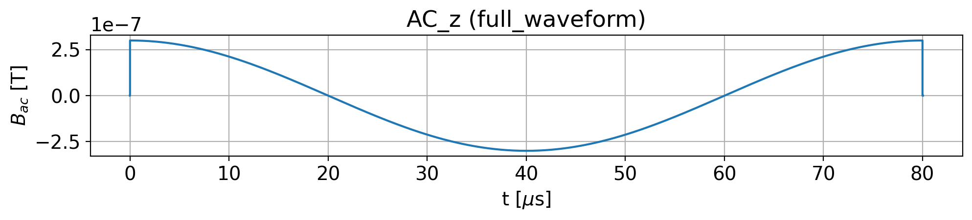
tau_values_n2 = np.linspace(5,35,41)
CPMG(model_n2, tau_res_n2, f_ac_mhz=frequency_target_n2, B_ac_tesla=B_ac_n2,
                             apply_noise=False, n_shots=1, n=2, plot=True)
signals_n2 = np.zeros(tau_values_n2.shape[0])
for idx, tau in enumerate(tau_values_n2):
    signals_n2[idx] = CPMG(model_n2, tau, f_ac_mhz=frequency_target_n2, B_ac_tesla=B_ac_n2,
                             apply_noise=False, n_shots=1, n=2)[0]
gamma_e_n2 = model_n2.spin('e').gyromagnetic_ratio  # MHz/T
tau_fine_n2 = np.linspace(tau_values_n2[0], tau_values_n2[-1], 400)
# minus sign: verified via an independent idealized qubit-rotation simulation (pi/2_x - pi_y(xn) - pi/2_x
# readout) that <ZI> = -cos(dPhi) for this pulse-axis sequence, for every n (not a scale effect, a fixed
# sign flip from the pulse-axis bookkeeping)
analytic_signal_n2 = -np.cos(delta_phi_analytic_cpmg(gamma_e_n2, B_ac_n2, frequency_target_n2, tau_fine_n2, n=2))

plt.plot(tau_values_n2, signals_n2, 'o-', label='simulated')
plt.plot(tau_fine_n2, analytic_signal_n2, '-', label='ideal analytic', alpha=0.7)
plt.axvline(tau_res_n2, color='r', linestyle='--', label=f'Resonance: {tau_res_n2:.1f} µs')
plt.legend()
plt.xlabel(r"$\tau$ [$\mu$s]")
plt.ylabel("<ZI>")
plt.title("AC sensing n = 2")
Text(0.5, 1.0, 'AC sensing n = 2')
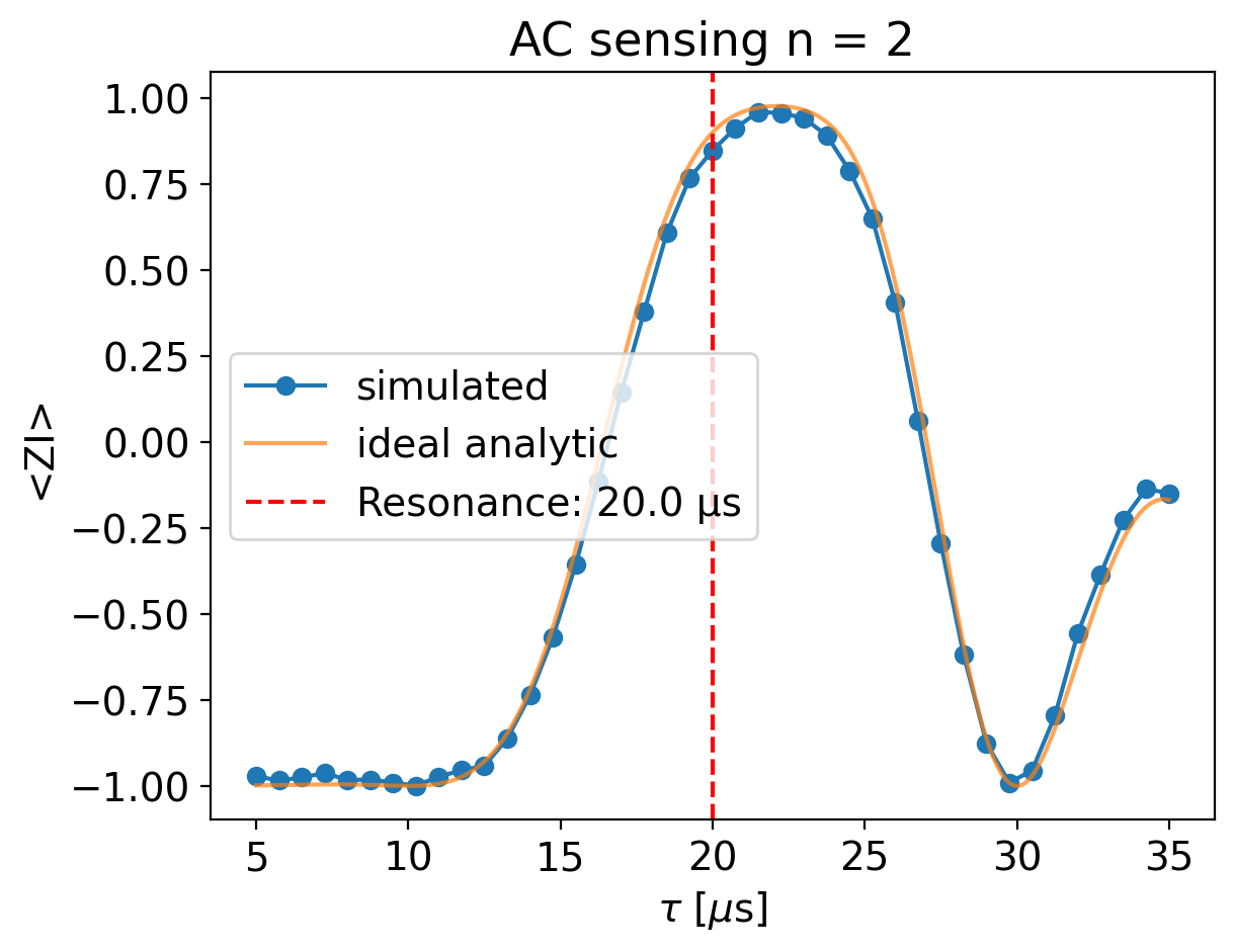
For \(n = 2\) the resonance is not much sharper than the Hahn echo. The total sensing time is \(T \approx 4\tau + 2t_{\pi}\), only twice the Hahn echo duration for the same \(\tau\), so the overhead of the two \(\pi/2\)-pulses is still comparable to the sensing part of the sequence.
Three \(\pi\)-pulses
model_n3 = simphony.default_nv_model(nitrogen_isotope=14, static_field_strength=B0)
outside_field_n3 = simphony.LinearDrivingField(
    direction=[0, 0, 1],
    name="AC_z"
)
model_n3.add_driving_field(outside_field_n3)
tau_res_n3 = 20
frequency_target_n3 = 1/(tau_res_n3*4+duration2)
B_ac_n3 = 3e-7
tau_values_n3 = np.linspace(5,35,61)
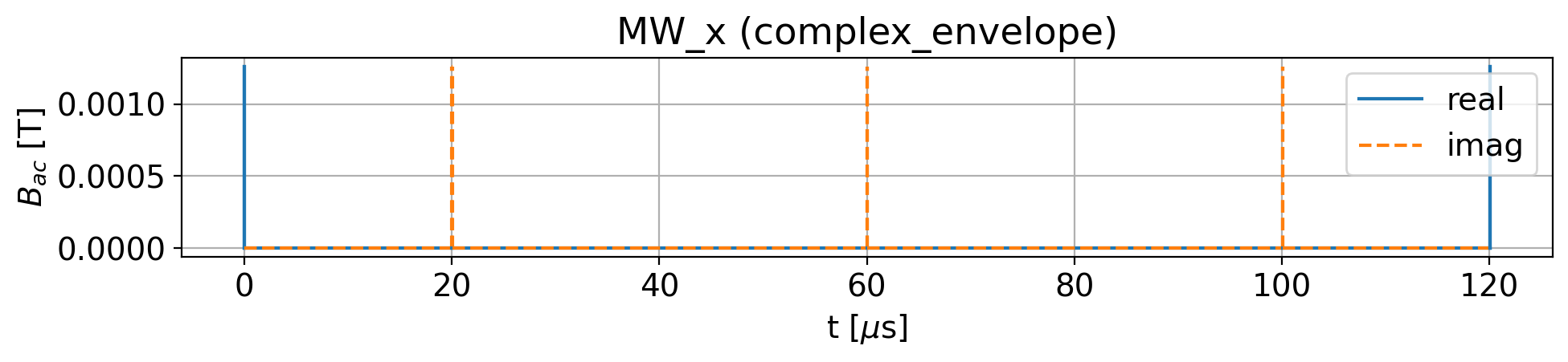
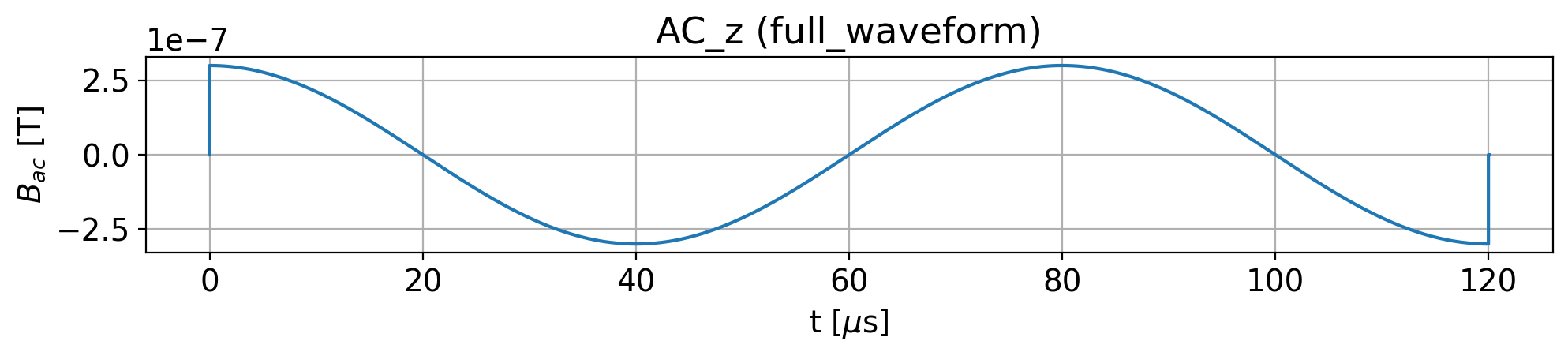
CPMG(model_n3, tau_res_n3, f_ac_mhz=frequency_target_n3, B_ac_tesla=B_ac_n3,
                             apply_noise=False, n_shots=1, n=3, plot=True)
signals_n3 = np.zeros(tau_values_n3.shape[0])
for idx, tau in enumerate(tau_values_n3):
    signals_n3[idx] = CPMG(model_n3, tau, f_ac_mhz=frequency_target_n3, B_ac_tesla=B_ac_n3,
                             apply_noise=False, n_shots=1, n=3)[0]
gamma_e_n3 = model_n3.spin('e').gyromagnetic_ratio  # MHz/T
tau_fine_n3 = np.linspace(tau_values_n3[0], tau_values_n3[-1], 400)
analytic_signal_n3 = -np.cos(delta_phi_analytic_cpmg(gamma_e_n3, B_ac_n3, frequency_target_n3, tau_fine_n3, n=3))

plt.plot(tau_values_n3, signals_n3, 'o-', label='simulated')
plt.plot(tau_fine_n3, analytic_signal_n3, '-', label='ideal analytic', alpha=0.7)
plt.axvline(tau_res_n3, color='r', linestyle='--', label=f'Resonance: {tau_res_n3:.1f} µs')
plt.legend()
plt.xlabel(r"$\tau$ [$\mu$s]")
plt.ylabel("<ZI>")
plt.title("AC sensing n = 3")
Text(0.5, 1.0, 'AC sensing n = 3')
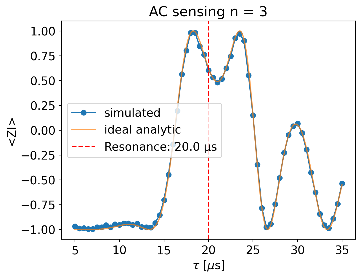
The central resonance is visibly narrower, and additional structure has appeared on either side of it. That structure is expected rather than spurious: once the accumulated phase exceeds \(2\pi\), \(\cos(\Delta\Phi)\) folds back on itself and the filter function develops sidelobes. The analytic curve reproduces them, which confirms they are signal.
Six \(\pi\)-pulses
model_n6 = simphony.default_nv_model(nitrogen_isotope=14, static_field_strength=B0)
outside_field_n6 = simphony.LinearDrivingField(
    direction=[0, 0, 1],
    name="AC_z"
)
model_n6.add_driving_field(outside_field_n6)
tau_res_n6 = 20
frequency_target_n6 = 1/(tau_res_n6*4+4*duration2)
B_ac_n6 = 3e-7
tau_values_n6 = np.linspace(10,30,61)
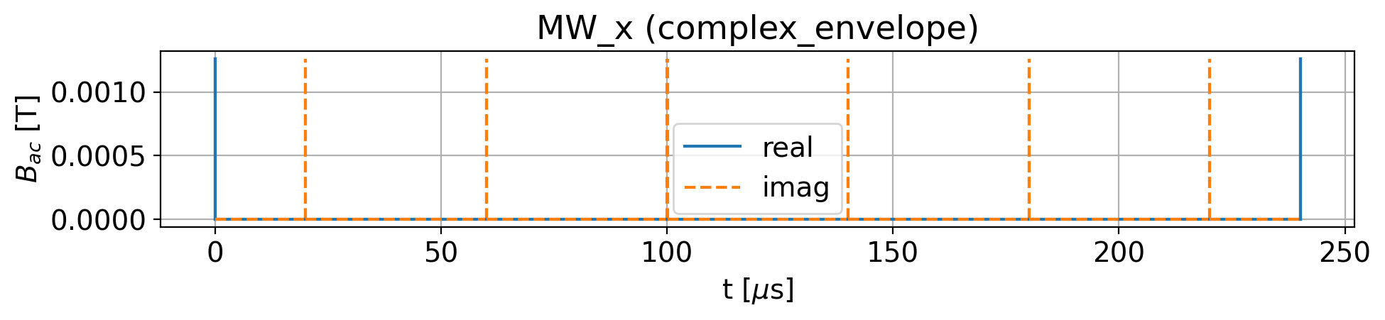
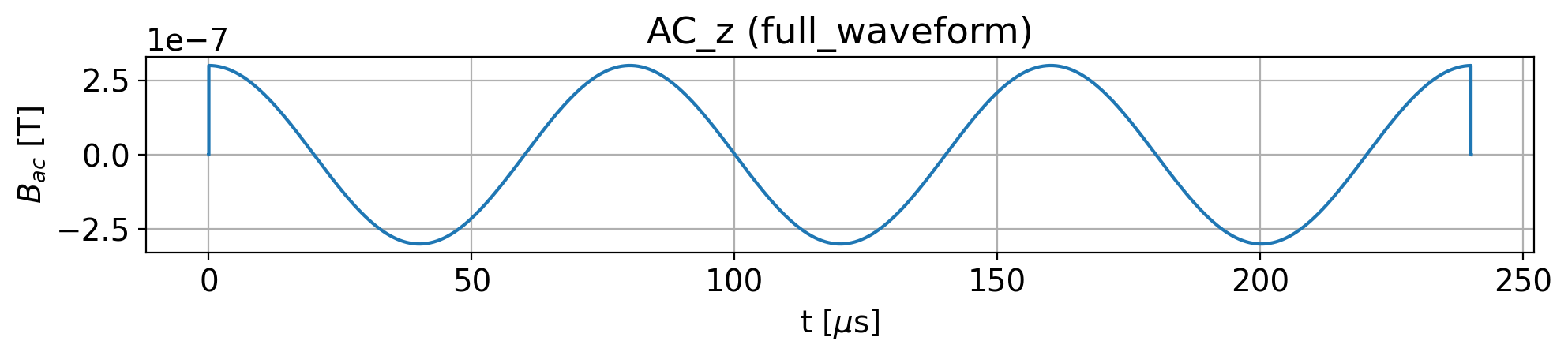
CPMG(model_n6, tau_res_n6, f_ac_mhz=frequency_target_n6, B_ac_tesla=B_ac_n6,
                             apply_noise=False, n_shots=1, n=6, plot=True)
signals_n6 = np.zeros(tau_values_n6.shape[0])
for idx, tau in enumerate(tau_values_n6):
    signals_n6[idx] = CPMG(model_n6, tau, f_ac_mhz=frequency_target_n6, B_ac_tesla=B_ac_n6,
                             apply_noise=False, n_shots=1, n=6)[0]
gamma_e_n6 = model_n6.spin('e').gyromagnetic_ratio  # MHz/T
tau_fine_n6 = np.linspace(tau_values_n6[0], tau_values_n6[-1], 400)
analytic_signal_n6 = -np.cos(delta_phi_analytic_cpmg(gamma_e_n6, B_ac_n6, frequency_target_n6, tau_fine_n6, n=6))

plt.plot(tau_values_n6, signals_n6, 'o-', label='simulated')
plt.plot(tau_fine_n6, analytic_signal_n6, '-', label='ideal analytic', alpha=0.7)
plt.axvline(tau_res_n6, color='r', linestyle='--', label=f'Resonance: {tau_res_n6:.1f} µs')
plt.legend()
plt.xlabel(r"$\tau$ [$\mu$s]")
plt.ylabel("<ZI>")
plt.title("AC sensing n = 6")
Text(0.5, 1.0, 'AC sensing n = 6')
Ten \(\pi\)-pulses
model_n10 = simphony.default_nv_model(nitrogen_isotope=14, static_field_strength=B0)
outside_field_n10 = simphony.LinearDrivingField(
    direction=[0, 0, 1],
    name="AC_z"
)
model_n10.add_driving_field(outside_field_n10)
tau_res_n10 = 20
frequency_target_n10 = 1/(tau_res_n10*4+8*duration2)
B_ac_n10 = 3e-7
tau_values_n10 = np.linspace(15,25,61)
CPMG(model_n10, tau_res_n10, f_ac_mhz=frequency_target_n10, B_ac_tesla=B_ac_n10,
                             apply_noise=False, n_shots=1, n=10, plot=True)
signals_n10 = np.zeros(tau_values_n10.shape[0])
for idx, tau in enumerate(tau_values_n10):
    signals_n10[idx] = CPMG(model_n10, tau, f_ac_mhz=frequency_target_n10, B_ac_tesla=B_ac_n10,
                             apply_noise=False, n_shots=1, n=10)[0]
gamma_e_n10 = model_n10.spin('e').gyromagnetic_ratio  # MHz/T
tau_fine_n10 = np.linspace(tau_values_n10[0], tau_values_n10[-1], 400)
analytic_signal_n10 = -np.cos(delta_phi_analytic_cpmg(gamma_e_n10, B_ac_n10, frequency_target_n10, tau_fine_n10, n=10))

plt.plot(tau_values_n10, signals_n10, 'o-', label='simulated')
plt.plot(tau_fine_n10, analytic_signal_n10, '-', label='ideal analytic', alpha=0.7)
plt.axvline(tau_res_n10, color='r', linestyle='--', label=f'Resonance: {tau_res_n10:.1f} µs')
plt.legend()
plt.xlabel(r"$\tau$ [$\mu$s]")
plt.ylabel("<ZI>")
plt.title("AC sensing n = 10")
Text(0.5, 1.0, 'AC sensing n = 10')
What the scans show
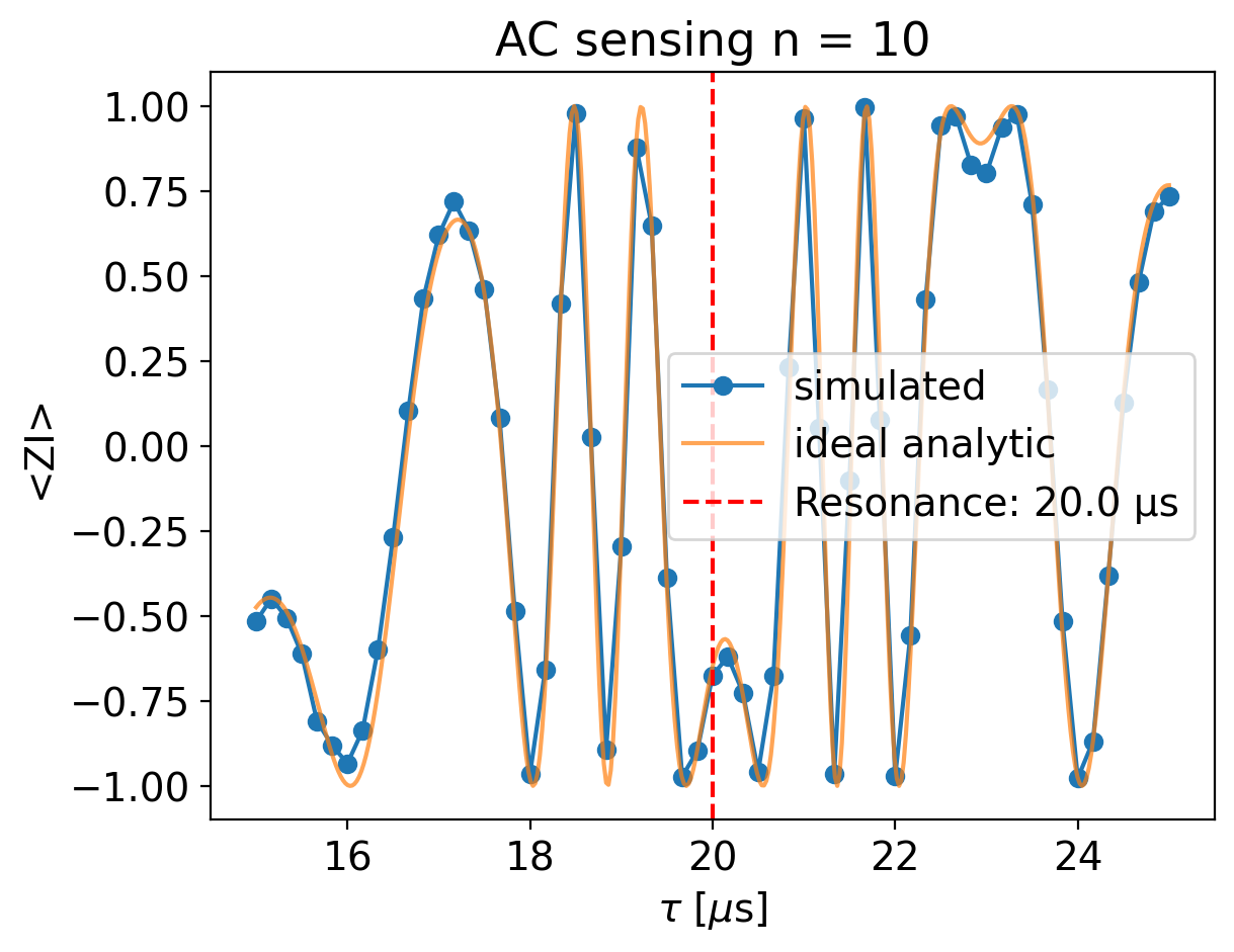
Three observations follow from the four scans above.
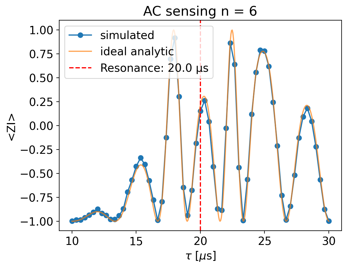
The resonance sharpens with \(n\). The central feature narrows steadily from \(n = 2\) to \(n = 10\), consistent with a sensing time \(T \approx 2n\tau\) and a filter function that narrows as \(1/n\). The next section measures this.
The sidelobes are real signal. The oscillations flanking the resonance become more numerous with \(n\), and the ideal instantaneous-pulse formula reproduces their position and shape at every \(n\). They come from the filter function folding through \(\cos(\Delta\Phi)\).
The agreement is good but not exact. At \(n = 6\) and \(n = 10\) some simulated extrema fall a few percent short of the analytic curve, which is the order of magnitude expected from the \(^{14}\)N hyperfine coupling that the two-level formula ignores.
Spectral resolution
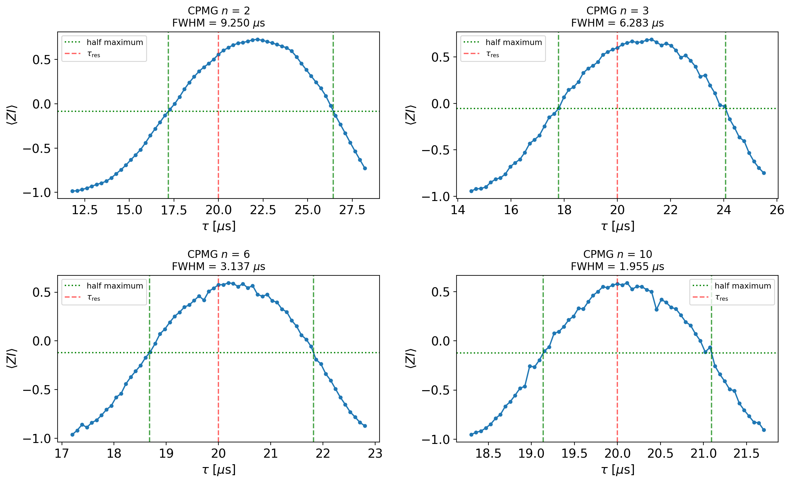
The practical value of CPMG is spectral resolution, quantified by the full width at half maximum of the resonance. The Fourier limit sets
with \(T \approx 2n\tau\) for CPMG(\(n\)), so the expected trend is \(\text{FWHM} \propto 1/n\).
Two points need care before measuring it.
The lineshape must not be folded. The signal is \(-\cos(\Delta\Phi)\), and once \(|\Delta\Phi|\) at resonance passes \(\pi\) the cosine folds back, breaking the \(\tau\) scan into several lobes of comparable size — at which point the width of “the” resonance is not defined. Scaling the AC amplitude as \(1/n\) holds the peak phase response fixed, so every sequence produces a single lobe with the same contrast and the widths are directly comparable.
The width must be extracted from the lineshape itself. The helper below locates the central extremum, takes a baseline from the scan wings, and returns the separation of the two linearly interpolated half-maximum crossings:
def resonance_fwhm(taus, signal, tau_res, search_frac=0.35):
    """FWHM of the central resonance, from linear-interpolated half-maximum crossings.

    The central feature is located as the extremum nearest ``tau_res``, the baseline is taken
    from the scan wings, and the width is the separation of the two points where the curve
    crosses half of (peak - baseline).

    Args:
        taus: Scanned free-evolution times (in us), monotonically increasing.
        signal: Corresponding <ZI> values.
        tau_res: Nominal resonance position, used to decide which extremum is the resonance.
        search_frac: Fraction of the scan span around ``tau_res`` searched for the extremum.

    Returns:
        Dict with the fwhm and the intermediate quantities needed to plot the measurement.
        ``fwhm`` is ``None`` if the scan window ends before the curve crosses the half level.
    """

    t = np.asarray(taus, dtype=float)
    s = np.asarray(signal, dtype=float)

    i_res = np.argmin(np.abs(t - tau_res))
    upward = s[i_res] > np.median(s)      # CPMG gives a peak here, the Hahn echo a dip
    ss = s if upward else -s

    near = np.abs(t - tau_res) <= search_frac * (t[-1] - t[0])
    i_peak = np.flatnonzero(near)[np.argmax(ss[near])]

    baseline = np.percentile(ss, 10)
    half = baseline + 0.5 * (ss[i_peak] - baseline)

    def crossing(indices):
        """First half-level crossing walking away from the peak; None if the scan ends first."""
        prev = i_peak
        for i in indices:
            if ss[i] < half:
                return t[prev] + (half - ss[prev]) * (t[i] - t[prev]) / (ss[i] - ss[prev])
            prev = i
        return None

    t_left = crossing(range(i_peak - 1, -1, -1))
    t_right = crossing(range(i_peak + 1, len(t)))

    fwhm = None if (t_left is None or t_right is None) else t_right - t_left
    sign = 1.0 if upward else -1.0

    return {'fwhm': fwhm, 'tau_left': t_left, 'tau_right': t_right,
            'half_level': sign * half, 'baseline': sign * baseline,
            'peak_tau': t[i_peak], 'peak_val': s[i_peak]}
Choosing the AC amplitude for each \(n\) so that the peak phase response is \(0.71\pi\) keeps all four sequences in the single-lobe regime:
# To compare linewidths across n we must keep every sequence in the single-lobe regime: once the
# accumulated phase at resonance passes pi, cos(dPhi) folds back and the tau scan develops several
# lobes of comparable size, at which point "the width of the resonance" is not defined. Scaling the
# AC amplitude as 1/n holds the peak phase response fixed, so all four sequences have the same
# contrast and the comparison is apples-to-apples.
def peak_phase(B_ac_tesla, f_ac_mhz, n, tau_res=20.0):
    """Accumulated phase at resonance for the ideal (instantaneous-pulse) CPMG(n) sequence."""
    return abs(delta_phi_analytic_cpmg(gamma_e_n6, B_ac_tesla, f_ac_mhz, tau_res, n=n))


f_ac_fwhm = 1 / (20 * 4 + 5 * duration2)
target_phase = 2.24                      # rad = 0.71 pi: single lobe, near-full contrast

# (n, tau window) -- windows sized to about 1.6x the expected width
fwhm_windows = {2: (11.8, 28.2), 3: (14.5, 25.5), 6: (17.2, 22.8), 10: (18.3, 21.7)}
fwhm_cfg = []
for n, window in fwhm_windows.items():
    B_ac_n = 1e-7 * target_phase / peak_phase(1e-7, f_ac_fwhm, n)
    fwhm_cfg.append((n, B_ac_n, window))

print(f'{"n":>3s}{"B_ac [T]":>13s}{"peak phase":>13s}{"tau window":>18s}')
for n, B_ac_n, window in fwhm_cfg:
    print(f'{n:3d}{B_ac_n:13.3e}{peak_phase(B_ac_n, f_ac_fwhm, n) / np.pi:11.2f} pi'
          f'{str(window):>18s}')
  n     B_ac [T]   peak phase        tau window
  2    2.499e-07       0.71 pi      (11.8, 28.2)
  3    1.666e-07       0.71 pi      (14.5, 25.5)
  6    8.330e-08       0.71 pi      (17.2, 22.8)
 10    4.999e-08       0.71 pi      (18.3, 21.7)
Now run the four scans:
# The four linewidth scans. Each uses its own AC amplitude and window from the cell above.
fwhm_scans = {}
for n, B_ac_n, window in fwhm_cfg:
    taus = np.linspace(window[0], window[1], 61)
    signal = np.zeros_like(taus)
    for idx, tau in enumerate(taus):
        model = simphony.default_nv_model(nitrogen_isotope=14, static_field_strength=B0)
        model.add_driving_field(simphony.LinearDrivingField(direction=[0, 0, 1], name='AC_z'))
        signal[idx] = CPMG(model, float(tau), f_ac_mhz=f_ac_fwhm, B_ac_tesla=B_ac_n,
                           apply_noise=False, n_shots=1, n=n)[0]
    fwhm_scans[n] = (taus, signal)
    print(f'n = {n:2d} done   range = [{signal.min():+.3f}, {signal.max():+.3f}]')
n = 2 done range = [-0.985, +0.728]
n = 3 done range = [-0.943, +0.689]
n = 6 done range = [-0.962, +0.595]
n = 10 done range = [-0.954, +0.591]
The construction is plotted alongside each scan, so the measurement can be checked by eye:
# Measure all four the same way, showing the construction so the reader can check it by eye.
fwhm_results = {}
fig, axes = plt.subplots(2, 2, figsize=(13, 8))
for ax, (n, (taus, signal)) in zip(axes.ravel(), sorted(fwhm_scans.items())):
    res = resonance_fwhm(taus, signal, tau_res=20.0)
    if res['fwhm'] is not None:
        fwhm_results[n] = res['fwhm']
    ax.plot(taus, signal, 'o-', markersize=3.5)
    ax.axhline(res['half_level'], color='g', linestyle=':', label='half maximum')
    for t_c in (res['tau_left'], res['tau_right']):
        if t_c is not None:
            ax.axvline(t_c, color='g', linestyle='--', alpha=0.7)
    ax.axvline(20.0, color='r', linestyle='--', alpha=0.6, label=r'$\tau_\mathrm{res}$')
    width = 'window too narrow' if res['fwhm'] is None else f"FWHM = {res['fwhm']:.3f} $\\mu$s"
    ax.set_title(f'CPMG $n$ = {n}\n{width}', fontsize=12)
    ax.set_xlabel(r'$\tau$ [$\mu$s]')
    ax.set_ylabel(r'$\langle ZI \rangle$')
    ax.legend(fontsize=9)
plt.tight_layout()
plt.show()

print(f'{"n":>3s}{"FWHM [us]":>12s}{"n x FWHM":>11s}')
for n in sorted(fwhm_results):
    print(f'{n:3d}{fwhm_results[n]:12.3f}{n * fwhm_results[n]:11.2f}')
  n   FWHM [us]   n x FWHM
  2       9.250      18.50
  3       6.283      18.85
  6       3.137      18.82
 10       1.955      19.55
ns = sorted(fwhm_results.keys())
fwhm_vals = [fwhm_results[n] for n in ns]

fig, axes = plt.subplots(1, 2, figsize=(13, 5))
axes[0].loglog(ns, fwhm_vals, 'o-', label='measured FWHM')
axes[0].loglog(ns, fwhm_vals[0] * ns[0] / np.array(ns, dtype=float), 'k--',
               label=r'$\propto 1/n$ reference')
axes[0].set_xlabel(r'number of $\pi$-pulses $n$')
axes[0].set_ylabel(r'FWHM($\tau$) [$\mu$s]')
axes[0].set_title('Spectral resolution vs. pulse number')
axes[0].legend()
axes[0].grid(True, which='both', alpha=0.3)

products = [n * w for n, w in zip(ns, fwhm_vals)]
axes[1].plot(ns, products, 'o-')
axes[1].axhline(np.mean(products), color='k', linestyle='--',
                label=f'mean = {np.mean(products):.2f} $\\mu$s')
axes[1].set_xlabel(r'number of $\pi$-pulses $n$')
axes[1].set_ylabel(r'$n \times$ FWHM [$\mu$s]')
axes[1].set_ylim(0, 1.5 * max(products))
axes[1].set_title(r'Constant $n \times$ FWHM confirms the $1/n$ law')
axes[1].legend()
axes[1].grid(alpha=0.3)
plt.tight_layout()
plt.show()

spread = (max(products) - min(products)) / np.mean(products)
print(f'n x FWHM = ' + ', '.join(f'{p:.2f}' for p in products) + ' us')
print(f'spread about the mean: {spread * 100:.1f}%')
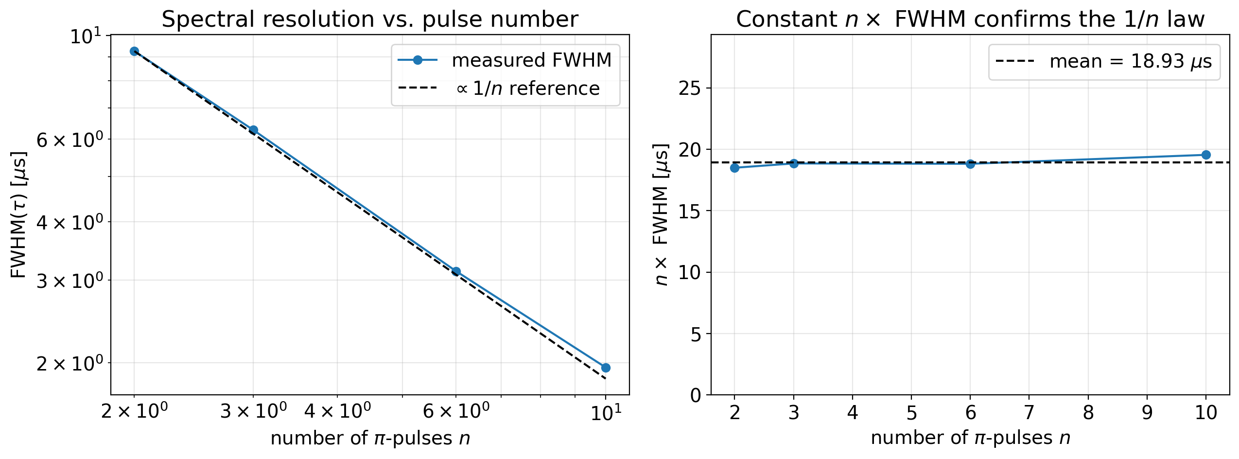
n x FWHM = 18.50, 18.85, 18.82, 19.55 us
spread about the mean: 5.5%
The \(1/n\) law
The measured FWHM falls monotonically with \(n\), and \(n \times \text{FWHM}\) is constant to a few percent — the Fourier-limit prediction \(\Delta f \approx 1/T\) with \(T \approx 2n\tau\), confirmed directly. Each additional \(\pi\)-pulse buys spectral resolution in proportion.
One caveat is worth recording. The simulated signal also carries a small, fast variation with \(\tau\), on scales far below the resonance width, which no ideal-pulse model contains. It comes from the finite rectangular \(\pi\)-pulses off-resonantly driving the \(|0\rangle \leftrightarrow |{+1}\rangle\) transition: the NV electron is a spin-1 system, and the second transition sits only \(2\gamma_e B_0 \approx 252\) MHz away from the \(25\) MHz Rabi drive. A little amplitude leaks into \(|{+1}\rangle\) on every pulse, accumulates phase while it is there, and interferes back at the next pulse. At the static field used here the effect is small enough not to disturb the linewidths above, and it is suppressed further at higher \(B_0\) — but it is the leading correction to the ideal-pulse picture, and it grows with the number of pulses.
Summary
In this notebook we simulated an AC magnetometry measurement with an NV center in Simphony:
The phase accumulated by the electron spin under a dynamical decoupling sequence was derived and expressed as an alternating-sign integral of the AC field.
A Hahn echo reproduced the AC resonance at \(f_{\text{AC}} = 1/(2\tau)\), matching the analytic filter-function prediction, and the phase scan showed the resonance can be located without prior knowledge of the AC phase.
CPMG sequences with \(n = 2, 3, 6, 10\) \(\pi\)-pulses narrowed the resonance progressively, with sidelobes that the ideal-pulse formula reproduces.
The spectral resolution improved as \(1/n\), with \(n \times \text{FWHM}\) constant to a few percent, as the Fourier limit requires.
The main departure from the ideal-pulse picture is off-resonant driving of the
\(|0\rangle \leftrightarrow |{+1}\rangle\) transition by the finite rectangular \(\pi\)-pulses, which
adds a small fast variation of the signal with \(\tau\) and accumulates with the number of pulses.
Suppressing it calls for either a larger static field or shaped pulses whose spectrum has less
weight at the unwanted transition — see the 3_tutorial_autodiff_gate_optimization notebook for
optimizing pulse shapes against gate infidelity with add_discrete_pulse() and
jax.value_and_grad.