Default NV model builders

The basic tutorial constructs a model that represents a nitrogen-vacancy (NV) center by hand. This tutorial uses the built-in NV models to construct the same kind of model.

The workflow is:

1. Start with the NV electron only.

2. Tilt the static magnetic field and compare quantization-axis choices.

3. Add the nitrogen nuclear spin.

4. Add selected carbon-13 spins from the hyperfine database.

5. Build two-NV models.

6. Compare same-orientation and different-orientation multi-NV models.

import numpy as np
import simphony

simphony.Config.set_matplotlib_format('retina')

Default single NV model

Simphony provides a built-in function to construct a default NV center model. Using the default_nv_model() function, you can define a model containing a single NV electron spin. When the levels are plotted, the spectrum shows the spin-1 electron levels in a relatively strong magnetic field:

model = simphony.default_nv_model(nitrogen_isotope=None,
                                  static_field_strength=0.05)

model.plot_levels()

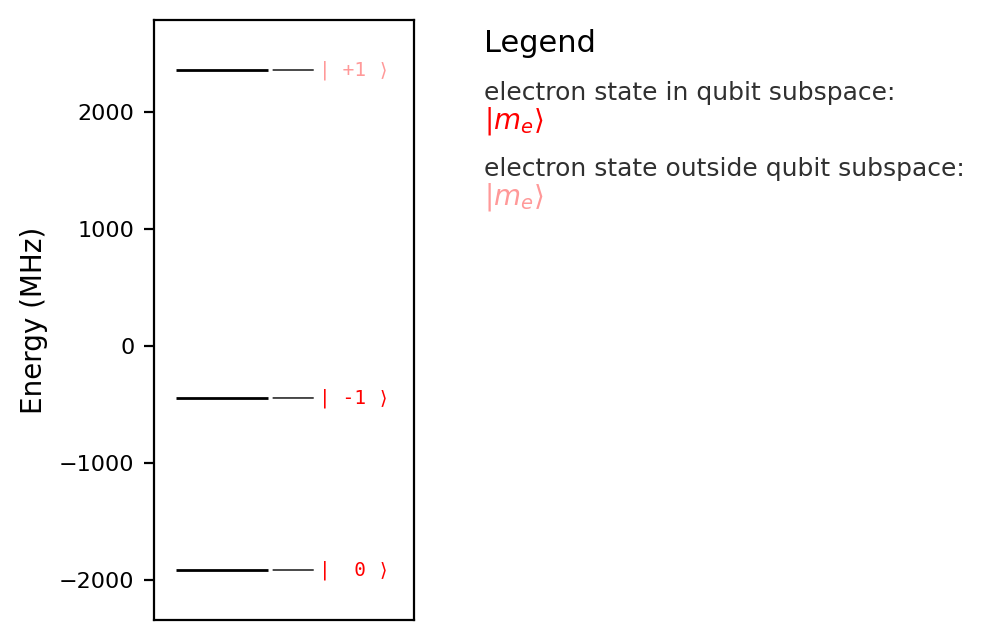
A single electron spin is attached to the model with the proper zero field splitting:

model.spins

[ElectronSpin(dimension=3, name='e', qubit_subspace=(0, -1), zero_field_splitting=2872.0)]

The crystallographic axis (we refer to this as anisotropy axis here) is hard-coded in the default_nv_model to point along the global z-axis:

model.spin('e').anisotropy_axis.vec

(0.0, 0.0, 1.0)

The default static field points along the z-axis too:

model.static_fields

[StaticField(strengths=(0.0, 0.0, 0.05))]

The builder also creates the standard MW and RF linearly polarized driving fields that point along the x-axis:

model.driving_fields

[LinearDrivingField(name='MW_x', direction=(1.0, 0.0, 0.0)),
 LinearDrivingField(name='RF_x', direction=(1.0, 0.0, 0.0))]

Tilted static magnetic field

With static_field_direction, you can tilt the direction of the static field, for example, by aligning with the x-axis:

model = simphony.default_nv_model(nitrogen_isotope=None,
                                  static_field_strength=0.2,
                                  static_field_direction=[1,0,0])

model.plot_levels()

/data/bope/codex_sandbox/simphony/simphony/model.py:1382: SimphonyWarning: Eigenstates are labelled via a one-to-one maximal-overlap assignment to local-S_z product-basis states. 3 assigned labels have overlap below 0.9:
eigenstate: - product state -> overlap
--------------------------------------
( 1.0): - ( 0.0) -> 0.376
        - ( 1.0) -> 0.312
        - (-1.0) -> 0.312
(-1.0): - (-1.0) -> 0.500
        - ( 1.0) -> 0.500
( 0.0): - ( 0.0) -> 0.624
        - (-1.0) -> 0.188
        - ( 1.0) -> 0.188
  warn(

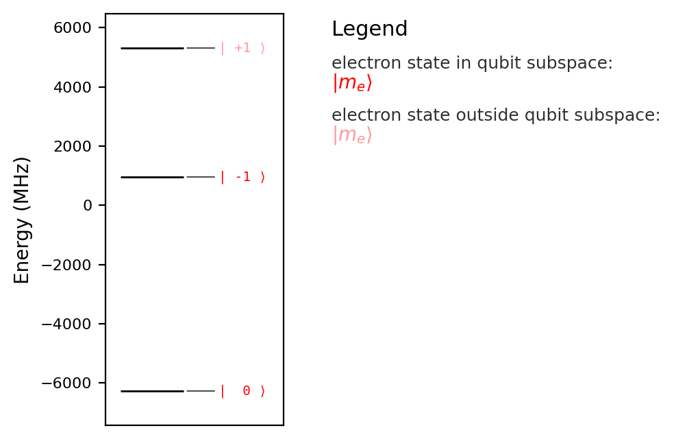
A labeling warning is expected here because the chosen basis does not align well with the eigenstates. In Simphony, eigenstate labeling is based on the overlap with the local-\(S_z\) eigenstates, or local-\(S_z\) product-basis states in the case of multiple spins, defined by the chosen quantization axis, using a one-to-one maximal-overlap assignment.

You can change the quantization_axis convention by choosing 'global_z', 'local_static_field', 'anisotropy_axis' or a general unit vector. In the current model, because the strong Zeeman term dominates the zero-field splitting term, we select 'local_static_field':

model = simphony.default_nv_model(nitrogen_isotope=None,
                                  static_field_strength=0.2,
                                  static_field_direction=[1,0,0],
                                  quantization_axis='local_static_field')

model.plot_levels()

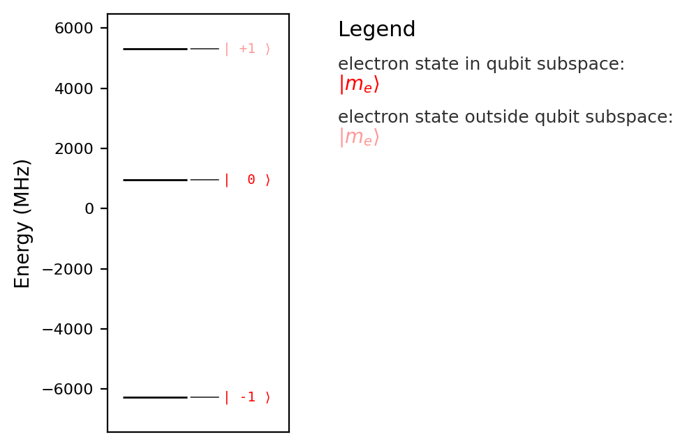
Overlaps between the eigenstates and local-\(S_z\) product-basis states can be checked by the model’s test_labeling() method:

model.test_labeling(output='print')

eigenstate: - product state -> overlap
--------------------------------------
(-1.0): - (-1.0) -> 0.984
        - ( 1.0) -> 0.016
( 1.0): - ( 1.0) -> 0.984
        - (-1.0) -> 0.016
( 0.0): - ( 0.0) -> 1.000

Now the eigenstate labels are dominated by a single local-\(S_z\) product-basis state. This is the diagnostic to use when a field or orientation choice makes the spectrum harder to label.

Add nitrogen and nearby carbon spins to the default model

A nitrogen nuclear spin can be added by specifying its isotope number through the nitrogen_isotope argument, which must be 14, 15, or None.

model = simphony.default_nv_model(nitrogen_isotope=14,
                                  static_field_strength=0.05)

model.plot_levels()

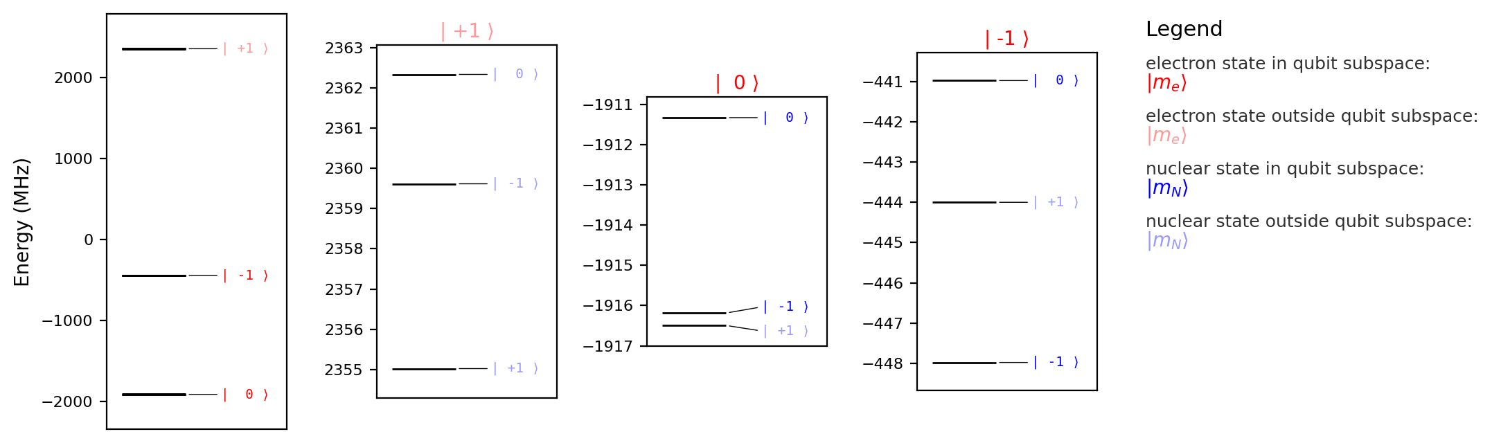
Additional carbon-13 nuclear spins can be included using the carbon_atom_indices argument to choose nuclear-spin sites and determine the hyperfine tensors, based on the Ivády Group’s hyperfine dataset. As mentioned above, the NV axis is aligned with the global z-direction.

The carbon_atom_indices must be a list of tuples. Each tuple \((n_1, n_2, n_3, n_4)\) defines the position of a carbon atom as:

\[ \text{carbon atom position} = n_1 \cdot \mathbf{a}_1 + n_2 \cdot \mathbf{a}_2 + n_3 \cdot \mathbf{a}_3 + n_4 \cdot \boldsymbol{\tau}, \]

where \(\mathbf{a}_1\), \(\mathbf{a}_2\), and \(\mathbf{a}_3\) are the primitive lattice vectors, and \(\mathbf{0}\) and \(\boldsymbol{\tau}\) are the positions of the carbon atoms inside the primitive cell. The indices \(n_1\), \(n_2\), \(n_3\) are integers, and \(n_4\) is either \(0\) or \(1\). Our convention is:

\[\begin{split} \begin{aligned} \mathbf{a}_1 &= a_\text{CC}\cdot \left( 0, \frac{2\sqrt{2}}{3}, \frac{4}{3} \right), \\ \mathbf{a}_2 &= a_\text{CC}\cdot \left( -\frac{\sqrt{6}}{3}, -\frac{\sqrt{2}}{3}, \frac{4}{3} \right), \\ \mathbf{a}_3 &= a_\text{CC}\cdot \left( \frac{\sqrt{6}}{3}, -\frac{\sqrt{2}}{3}, \frac{4}{3} \right), \\ \boldsymbol{\tau} &= \frac{\mathbf{a}_1 + \mathbf{a}_2 + \mathbf{a}_3}{4} = a_\text{CC}\cdot (0, 0, 1), \end{aligned} \end{split}\]

where \(a_\text{CC} = 0.1545\ \text{nm}\) is the carbon–carbon distance. The nitrogen occupies the \(\boldsymbol{\tau}\) position, while the missing carbon atom (vacancy) corresponds to the \(\mathbf{0}\) lattice point.

The spin-Hamiltonian describes the default NV model:

\[ H = \underbrace{\gamma_{e} \mathbf{B} \cdot \mathbf{S} + D S_z^2}_{\text{electron}} + \underbrace{-\gamma_{N} \mathbf{B} \cdot \mathbf{I}_{N} + P I_{N,z}^2 + \mathbf{S} \cdot \mathbf{A}_{N} \cdot \mathbf{I}_{N}}_{\text{nitrogen}} + \underbrace{\sum_{i} \left(-\gamma_{C} \mathbf{B} \cdot \mathbf{I}_{C}^{(i)} + \mathbf{S} \cdot \mathbf{A}_{C}^{(i)} \cdot \mathbf{I}_{C}^{(i)} \right)}_{\text{carbon(s)}}. \]

Spin	Parameter	Symbol	Value
Electron \((S=1)\)	Gyromagnetic ratio	\(γ_e\)	28.0331 GHz/T [1]
	Zero-field splitting	\(D\)	2.872 GHz [1]
Nitrogen-14 \((I=1)\)	Gyromagnetic ratio	\(γ_N\)	3.07771 MHz/T [2]
	Quadrupole splitting	\(P\)	-5.01 MHz [1]
	Hyperfine perpendicular	\(A_{N\perp}\)	-2.70 MHz [1]
	Hyperfine parallel	\(A_{N\parallel}\)	-2.14 MHz [1]
Nitrogen-15 \((I=1/2)\)	Gyromagnetic ratio	\(γ_N\)	-4.31727 MHz/T [2]
	Hyperfine perpendicular	\(A_{N\perp}\)	3.65 MHz [1]
	Hyperfine parallel	\(A_{N\parallel}\)	3.03 MHz [1]
Carbon-13 \((I=1/2)\)	Gyromagnetic ratio	\(γ_C\)	10.7084 MHz/T [2]

References:

[1] Felton et al., Phys. Rev. B 79, 075203 (2009)
[2] CRC Handbook of Chemistry and Physics, sec. 11-4 (97th edition)

A simple spin system consisting of an NV electron spin, a \(^{14}\text{N}\) nuclear spin, and two \(^{13}\text{C}\) nuclear spins can be defined as:

model = simphony.default_nv_model(nitrogen_isotope=14,
                                  carbon_atom_indices=[(1,1,1,0),(2,-3,4,1)],
                                  static_field_strength=0.05)

model.plot_levels()

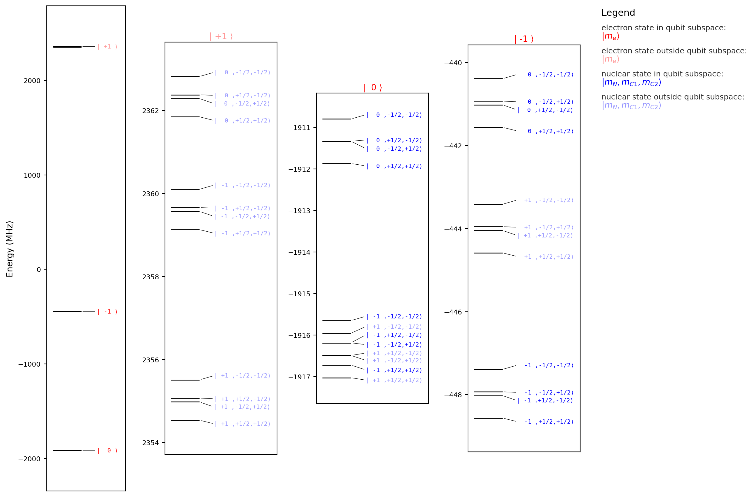
The resulting model contains four attached spins and three spin-spin interactions, as expected for this electron-nitrogen-two-carbon system:

model.spins

[ElectronSpin(dimension=3, name='e', qubit_subspace=(0, -1), zero_field_splitting=2872.0),
 NuclearSpin(dimension=3, name='N', qubit_subspace=(0, -1), quadrupole_splitting=-5.01),
 NuclearSpin(dimension=2, name='C1', qubit_subspace=(-0.5, 0.5)),
 NuclearSpin(dimension=2, name='C2', qubit_subspace=(-0.5, 0.5))]

model.interactions

[Interaction(spin_name_1='e', spin_name_2='N', diag=[-2.7, -2.7, -2.14], offdiag='zero'),
 Interaction(spin_name_1='e', spin_name_2='C1', diag=[-0.06727, -0.06727, 0.095884], offdiag='approx_zero'),
 Interaction(spin_name_1='e', spin_name_2='C2', diag=[0.005059, -0.009612, 0.004552], offdiag='nonzero')]

By default, each default NV model includes a RotatingFrameSetter, which recomputes the rotating-frame frequency of each spin from its current qubit splitting whenever the model parameters change. The default configuration uses rest_electron_spin_state='1' and rest_nuclear_spin_state='avg': when the rotating-frame frequency of one spin is computed, Simphony calculates that spin’s qubit splitting while fixing the other electron spins to qubit state '1' and averaging over the other nuclear spins:

model.rotating_frame

RotatingFrameSetter(rest_electron_spin_state='1', rest_nuclear_spin_state='avg')

The default qubit subspaces corresponding the spins are:

{spin.name: spin.qubit_subspace for spin in model.spins}

{'e': (0, -1), 'N': (0, -1), 'C1': (-0.5, 0.5), 'C2': (-0.5, 0.5)}

That can be changed easily at initialization by the qubit_subspace_electron, qubit_subspace_nitrogen and qubit_subspace_carbon arguments. The qubit subspace defines which two local spin states are treated as the computational states of each spin, so setting it explicitly makes later gate simulations and pulse-design examples unambiguous.

Hyperfine database

The hyperfine database can be accessed directly by:

db = simphony.default_nv_hyperfine_database()
len(db)

19924

The database contains information regarding site indices, positions (both ideal and DFT), occupied atoms, and \(^{13}\text{C}\) hyperfine interactions:

db[:3]

(NVLatticeSite(
   type='N',
   index=(0, 0, 0, 1),
   hyperfine=nan,
   lattice_positions=(1.11022e-16, -2.498e-16, 0.772278),
   dft_positions=(4.35002e-06, 2.60769e-06, 0.93198),
   distance_from_lattice_center=0.772278,
 ),
 NVLatticeSite(
   type='V',
   index=(0, 0, 0, 0),
   hyperfine=nan,
   lattice_positions=(0, 0, -0.772278),
   dft_positions=(0, -4.44089e-16, -0.772278),
   distance_from_lattice_center=0.772278,
 ),
 NVLatticeSite(
   type='C',
   index=(-1, 0, 0, 1),
   hyperfine=(
     (109.921, -0.000324996, -0.000111407),
     (-0.000324996, 187.35, 25.4812),
     (-0.000111407, 25.4812, 117.999),
   ),
   lattice_positions=(-1.05407e-17, -1.45622, -1.28713),
   dft_positions=(5.59251e-06, -1.53528, -1.34177),
   distance_from_lattice_center=1.94352,
 ))

Build coupled NV-center models

Function default_multi_nv_model() extends the builder to several NV centers. In this example, dipole-dipole coupled NV centers are created with the same crystallographic orientation and without nuclear spins. The orientation should be one of (1, 1, 1), (1, -1, -1), (-1, 1, -1), or (-1, -1, 1), representing the possible crystallographic axes of NV centers in diamond. The positions of the NV centers are passed through the positions argument, given in \(\text{nm}\):

model = simphony.default_multi_nv_model(orientations=[(1,1,1),(1,1,1)],
                                        positions=[[0,0,0],[1,3,10]],
                                        nitrogen_isotopes=None,
                                        static_field_strengths=[0.01,0.0101])

model.plot_levels()
model.spin_names

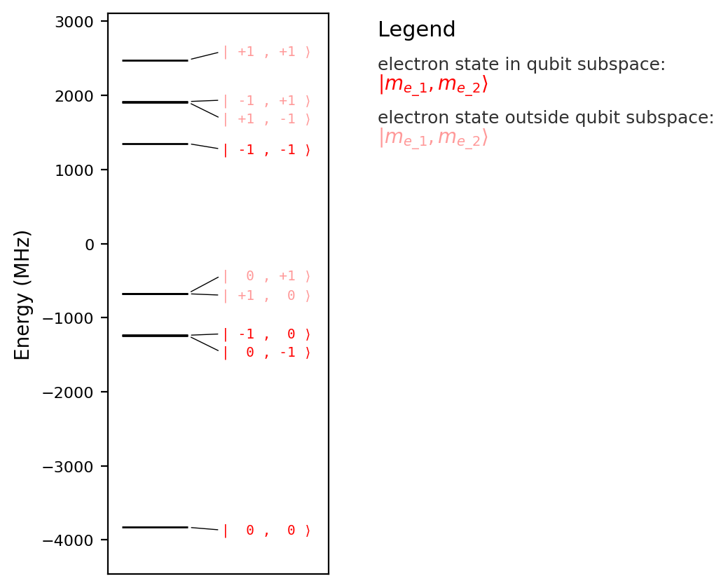
['e_1', 'e_2']

Passing a list to static_field_strengths creates separate static fields for the spins:

model.static_fields

[StaticField(strengths=(0.0, 0.0, 0.01), target_spins=('e_1',)),
 StaticField(strengths=(0.0, 0.0, 0.0101), target_spins=('e_2',))]

The previous model used two different field strengths, so the builder created targeted static fields rather than one global field. The target list tells which spins each field acts on. This matters later when a model contains electron and nuclear spins from several centers: a field or drive can be global, or it can be restricted to one part of the register. A scalar static_field_strengths value creates one global field; a list creates targeted fields for the corresponding centers.

Two NV centers with different orientations

Now the second NV center is placed along a different crystallographic orientation. With the default quantization convention, both electron spins are still represented in the global-z basis even though their anisotropy axes differ, which leads to problematic labeling:

model = simphony.default_multi_nv_model(orientations=[(1,1,1),(1,-1,-1)],
                                        positions=[[0,0,0],[1,3,10]],
                                        nitrogen_isotopes=None,
                                        static_field_strengths=0.01)

model.plot_levels()
model.spin_names

/data/bope/codex_sandbox/simphony/simphony/model.py:1382: SimphonyWarning: Eigenstates are labelled via a one-to-one maximal-overlap assignment to local-S_z product-basis states. 9 assigned labels have overlap below 0.9:
eigenstate: - product state -> overlap
--------------------------------------
( 1.0,  0.0): - ( 1.0,  0.0) -> 0.531
              - ( 1.0, -1.0) -> 0.360
              - ( 1.0,  1.0) -> 0.108
( 1.0,  1.0): - ( 1.0,  1.0) -> 0.531
              - ( 1.0,  0.0) -> 0.360
              - ( 1.0, -1.0) -> 0.108
( 1.0, -1.0): - ( 1.0, -1.0) -> 0.531
              - ( 1.0,  1.0) -> 0.360
              - ( 1.0,  0.0) -> 0.108
( 0.0,  1.0): - ( 0.0,  1.0) -> 0.531
              - ( 0.0,  0.0) -> 0.360
              - ( 0.0, -1.0) -> 0.108
( 0.0, -1.0): - ( 0.0, -1.0) -> 0.531
              - ( 0.0,  1.0) -> 0.360
              - ( 0.0,  0.0) -> 0.108
( 0.0,  0.0): - ( 0.0,  0.0) -> 0.531
              - ( 0.0, -1.0) -> 0.360
              - ( 0.0,  1.0) -> 0.108
(-1.0, -1.0): - (-1.0, -1.0) -> 0.531
              - (-1.0,  1.0) -> 0.360
              - (-1.0,  0.0) -> 0.108
(-1.0,  1.0): - (-1.0,  1.0) -> 0.531
              - (-1.0,  0.0) -> 0.360
              - (-1.0, -1.0) -> 0.108
(-1.0,  0.0): - (-1.0,  0.0) -> 0.531
              - (-1.0, -1.0) -> 0.360
              - (-1.0,  1.0) -> 0.108
  warn(

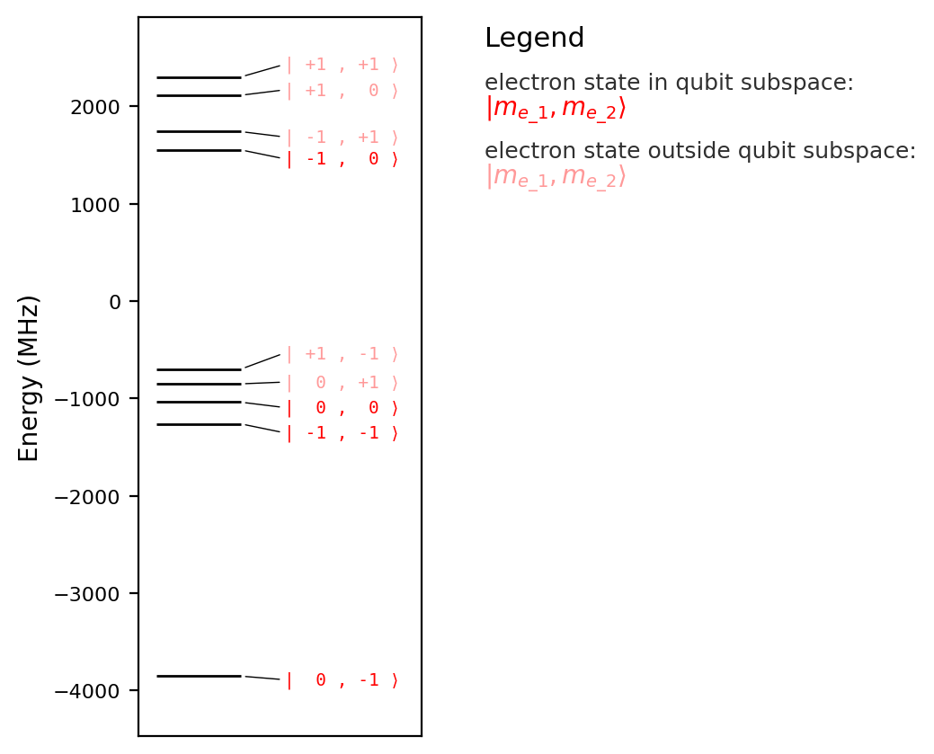
['e_1', 'e_2']

Using quantization_axis='anisotropy_axis' makes each spin’s local basis follow its own NV axis. For multi-orientation models this is often the clearer convention, because the basis now follows the physical principal axis of each center:

model = simphony.default_multi_nv_model(orientations=[(1,1,1),(1,-1,-1)],
                                        positions=[[0,0,0],[1,10,3]],
                                        nitrogen_isotopes=None,
                                        static_field_strengths=0.01,
                                        quantization_axis='anisotropy_axis')

model.plot_levels()
model.spin_names

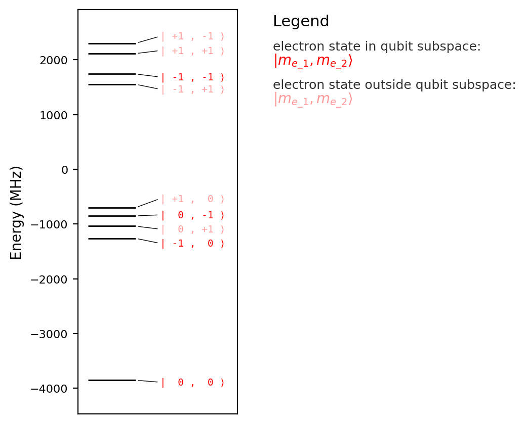
['e_1', 'e_2']

Overlaps between the eigenstates and local-\(S_z\) product-basis states can be visualized by the model’s test_labeling(output='plot') method:

model.test_labeling(output='plot')

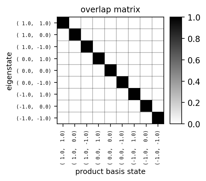
Strong diagonal weight means the assigned labels are easy to interpret.

Summary

The default NV builders provide a compact way to construct physically parameterized NV models:

• default_nv_model() creates a single NV-center model.

• nitrogen_isotope adds the nitrogen nuclear spin.

• carbon_atom_indices selects carbon-13 sites from the hyperfine database.

• static_field_direction changes the magnetic-field orientation.

• quantization_axis controls the basis used for state labels and labeling diagnostics.

• default_multi_nv_model() adds NV-center orientations, positions, local fields, and multi-center interactions.

Use plot_levels() to compare spectra after each modeling choice, and use test_labeling() when the basis or geometry may make state labels ambiguous.