Pulsed ODMR
Optically detected magnetic resonance (ODMR) is the most basic NV measurement: the electron spin is optically initialized, a microwave pulse at some frequency \(f\) is applied, and the population left in the \(m_S=0\) electron spin state is read out optically. Sweeping \(f\) traces out a resonance spectrum — this is usually the very first measurement in any NV experiment, since it locates the resonance frequencies that every other pulse sequence (Rabi, Ramsey, …) depends on.
In pulsed ODMR, the microwave pulse has a fixed, finite duration \(\tau\), applied with the laser off (unlike continuous-wave ODMR, where laser and microwave are on simultaneously). Simphony does not currently model the optical initialization/readout physics directly, so reading out the population in \(m_S=0\) simply means evaluating the \(m_S=0\) population at the end of the pulse.
A real ODMR measurement does not initialize the nuclear spin state between shots — it is
effectively thermally unpolarized. Rather than assuming one fixed nuclear spin projection, we capture
this by initializing the model in a mixed state via Model.initial_density_matrix. With the
\(^{14}\mathrm{N}\) nuclear spin, this naturally produces the classic hyperfine-resolved triplet:
three resonance dips, one per nuclear spin projection \(m_I\), each broadened by the pulse’s finite
duration.
We assume familiarity with the components, pulses, and simulation workflow introduced in the basic tutorial.
Import the packages
import numpy as np
import matplotlib.pyplot as plt

import simphony

simphony.Config.set_platform('cpu')
simphony.Config.set_matplotlib_format('retina')
Model
We use the electron + \(^{14}\mathrm{N}\) system (dimension 3 nuclear spin, spin projection \(m_I \in \{-1, 0, +1\}\)), which has default MW_x/RF_x driving fields already attached. The model’s built-in hyperfine splitting (\(2.14\) MHz) is close to the \(2.16\) MHz value measured by Dréau et al., “Avoiding power broadening in optically detected magnetic resonance of single NV defects for enhanced dc magnetic field sensitivity”, Phys. Rev. B 84, 195204 (2011), for a real \(^{14}\mathrm{N}\) NV defect:
model = simphony.default_nv_model(nitrogen_isotope=14)
model
Model(spin_names=['e', 'N'], num_static_fields=1, driving_field_names=['MW_x', 'RF_x'], dimension=9)
A thermally unpolarized nuclear spin
Since the nuclear spin state is not initialized, we model it as maximally mixed, \(\rho_N = I_3 / 3\), with the electron optically initialized into \(m_S=0\):
initial_density_matrix = sum(
    (1 / 3) * np.outer(state, state.conjugate())
    for state in (model.productstate({'e': 0, 'N': m_I}) for m_I in (-1, 0, 1))
)
Pulsed-ODMR sweep
We sweep the pulse frequency and, at each point, apply a single rectangle pulse whose amplitude is chosen so that a resonant pulse of the given duration implements a full \(\pi\) rotation (experimentally, this amplitude would likewise be found by first calibrating a Rabi oscillation at that specific duration, exactly as rabi_amplitude_qubit does here numerically). This keeps on-resonance contrast maximal regardless of duration, so any change in the resulting spectrum’s width is not confounded by a change in pulse area.
For the readout operator, we use the built-in 'M' symbol: the full-space projector onto \(m_S=0\), paired with '1' (identity) for the nuclear spin so that all three nuclear spin projections \(m_I\) are included. (The nuclear spin is named 'N' in the model — the string key used below in rest_quantum_nums={'N': ...} — while \(m_I\) is its physical spin-projection quantum number.) This directly matches how a real ODMR trace is normally read and plotted: a population between \(0\) and \(1\):
def pulsed_odmr(model, duration, frequencies, initial_density_matrix):
    angle = np.pi
    period_time = 2 * np.pi * duration / angle  # = 2 * duration
    amplitude = model.rabi_amplitude_qubit(driving_field_name='MW_x',
                                           period_time=period_time,
                                           spin_name='e')

    contrasts = []
    for frequency in frequencies:
        model.remove_all_pulses()
        model.driving_field('MW_x').add_rectangle_pulse(amplitude=amplitude,
                                                        frequency=frequency,
                                                        phase=0,
                                                        duration=duration)

        result = model.simulate_time_evolution(n_eval=2)
        result.initial_density_matrix = initial_density_matrix
        contrast = result.expectation_value('M1',
                                            t_idx=-1,
                                            source='density_matrix',
                                            frame='lab',
                                            in_qubit_subspace=False)
        contrasts.append(contrast[0, 0, 0])

    return np.array(contrasts)
We center the frequency sweep on the average electron splitting and scan a window wide enough to cover all three hyperfine branches. For the pulse duration, we pick duration_long = 3.6 \(\mu\text{s}\), very close to the coherence time \(T_2^* = 3.0 \pm 0.2\) \(\mu\text{s}\) measured by Dréau et al. — not an arbitrarily long pulse, but close to the real experimental “sweet spot.” This corresponds to a Rabi frequency of about \(0.139\) MHz (1 / (2 * 3.6 us)), well below the ~2.14 MHz hyperfine splitting, so its Fourier bandwidth shouldn’t blur the three branches together:
splitting_center = model.splitting_qubit('e')
frequencies = splitting_center + np.linspace(-5, 5, 201)  # MHz

duration_long = 3.6  # us, close to the T_2^* = 3.0 us measured by Dreau et al. (2011)
contrast_long = pulsed_odmr(model, duration_long, frequencies, initial_density_matrix)

plt.plot(frequencies, contrast_long)
plt.xlabel('MW frequency (MHz)')
plt.ylabel('population in $m_S=0$')
plt.title(f'Pulsed ODMR, duration = {duration_long} us')
plt.show()
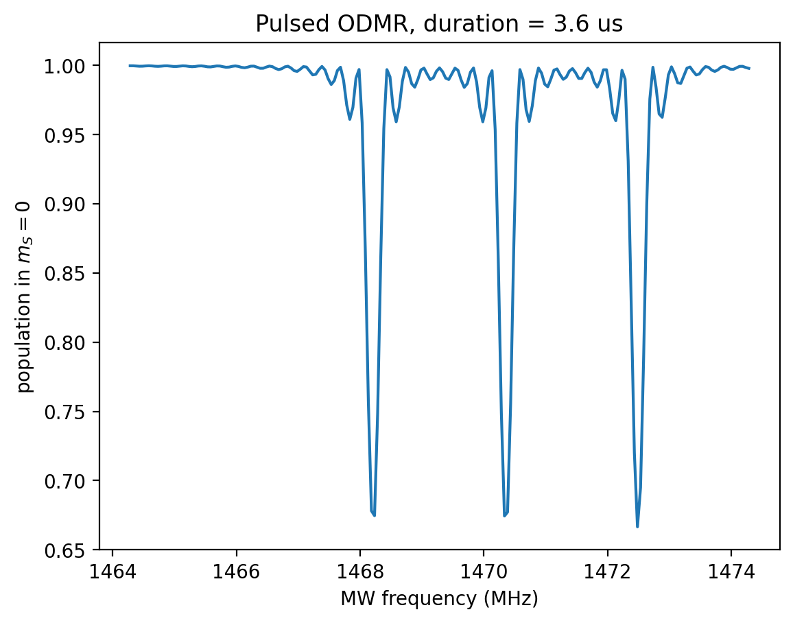
The three dips sit at the electron splitting conditioned on each nuclear spin projection \(m_I\). We can check the predicted locations directly:
for m_I in (-1, 0, 1):
    splitting_m_I = model.splitting_qubit('e', rest_quantum_nums={'N': m_I})
    print(f'm_I={m_I:+d}: predicted dip at {splitting_m_I:.4f} MHz')
m_I=-1: predicted dip at 1468.2099 MHz
m_I=+0: predicted dip at 1470.3566 MHz
m_I=+1: predicted dip at 1472.4917 MHz
Only one nuclear spin projection \(m_I\) is resonant at each dip, so only \(1/3\) of the population is driven out of \(m_S=0\) there, while the other \(2/3\) stays near population \(1\). The predicted dip minimum is therefore
which we can compare against the simulated minimum:
print(f'simulated dip minimum  = {contrast_long.min():.4f}')
print(f'predicted dip minimum   = {2/3:.4f}')
simulated dip minimum  = 0.6665
predicted dip minimum   = 0.6667
Pulse-duration-limited linewidth
A much shorter pulse delivers the same \(\pi\)-rotation area with proportionally higher amplitude, and its Fourier bandwidth exceeds the ~2.14 MHz hyperfine splitting — the three lines (one per \(m_I\)) broaden and merge. We pick duration_short = 0.45 \(\mu\text{s}\), corresponding to a Rabi frequency of about 1.1 MHz (1 / (2 * 0.45 us)):
duration_short = 0.45  # us, a short pi-pulse well below T_2^* (Dreau et al. 2011)
contrast_short = pulsed_odmr(model, duration_short, frequencies, initial_density_matrix)

plt.plot(frequencies, contrast_long, label=f'duration = {duration_long} us')
plt.plot(frequencies, contrast_short, label=f'duration = {duration_short} us')
plt.xlabel('MW frequency (MHz)')
plt.ylabel('population in $m_S=0$')
plt.title('Pulse-duration-limited ODMR linewidth')
plt.legend()
plt.show()
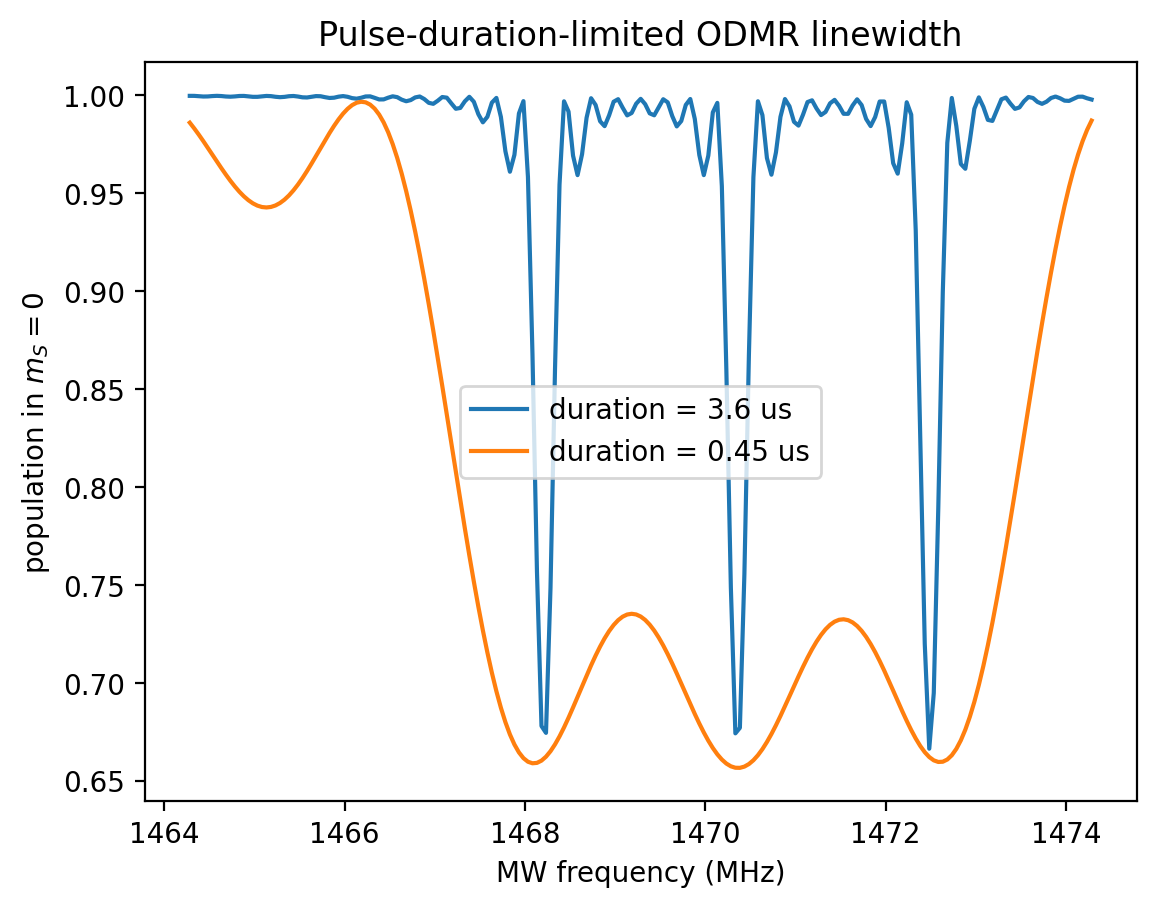
fourier_bandwidth_short = 1 / duration_short
adjacent_hyperfine_splitting = (model.splitting_qubit('e', rest_quantum_nums={'N': 0})
                                - model.splitting_qubit('e', rest_quantum_nums={'N': -1}))

print(f'Fourier bandwidth ~ 1 / duration_short      = {fourier_bandwidth_short:.3f} MHz')
print(f'adjacent hyperfine splitting (m_I=-1 to 0)  = {adjacent_hyperfine_splitting:.3f} MHz')
Fourier bandwidth ~ 1 / duration_short      = 2.222 MHz
adjacent hyperfine splitting (m_I=-1 to 0)  = 2.147 MHz
As predicted, the Fourier bandwidth is slightly larger than the adjacent hyperfine splitting — enough to blur the three branches together into the single broadened line seen above.
This is the practical reason pulse duration must be chosen carefully in pulsed ODMR: a pulse short enough to be convenient can broaden the resonance past the hyperfine splitting, hiding structure that a longer (but still finite) pulse resolves cleanly.
This is exactly the effect exploited by Dréau et al. (2011): replacing continuous-wave ODMR with a resonant microwave \(\pi\)-pulse followed by an optimized readout pulse removes power broadening from the linewidth, since the pulse’s own (finite) duration — not the drive amplitude — then sets the resolution.
A caveat: in the real experiment, the linewidth does not keep narrowing forever as \(T_\pi\) grows. Dréau et al. measure the linewidth becoming Fourier-limited (\(\propto 1/T_\pi\)) for \(T_\pi \ll T_2^*\), but then saturating around \(\Gamma_2^* \approx 0.2\) MHz once \(T_\pi \gtrsim T_2^* = 3.0\) \(\mu\text{s}\), with the contrast then degrading for still-longer pulses instead of the line narrowing further. This simulation has no \(T_2^*\)/dephasing mechanism, so it cannot reproduce that saturation — an arbitrarily long duration here would keep narrowing the simulated line indefinitely. duration_long = 3.6 \(\mu\text{s}\) is chosen close to the paper’s measured \(T_2^*\), matching the regime where their observed saturation sets in.
Summary
A pulsed-ODMR spectrum is a frequency-swept \(\pi\)-pulse experiment, naturally expressed with the same pulse-construction tools (
add_rectangle_pulse,rabi_amplitude_qubit) used throughout the tutorial series.A real ODMR measurement does not know the nuclear-spin state; representing it as a thermally mixed
Model.initial_density_matrixreproduces the hyperfine-resolved triplet directly from a single frequency sweep, including the reduced (\(2/3\) population, i.e. \(1/3\) fractional contrast) per-line dip depth from branching over the three nuclear spin projections \(m_I \in \{-1,0,+1\}\).The built-in
'M'operator string symbol (paired with'1'for spectator spins) reads out the full-space \(m_S=0\) population directly, avoiding the need to reason about qubit-subspace truncation for spins with more physical levels than their addressed qubit subspace.The ODMR linewidth is limited by the microwave pulse duration (Fourier/power broadening): a longer \(\pi\)-pulse resolves hyperfine structure that a shorter one of the same pulse area blurs together.