DC magnetometry and robust-pulse optimization with an NV center
One of the best-known applications of the NV center is as a magnetometer: its electron-spin resonance shifts with an applied magnetic field (Zeeman effect), so measuring that shift reveals the field. This notebook has three parts.
Part 1 measures a static (DC) field with a Ramsey sequence, reads it out by slope detection, and defines the figure of merit a magnetometer is judged by, the sensitivity \(\eta\).
Part 2 moves from one spin to an ensemble, as real diamond magnetometers do to sense with many spins at once. Packing NV centres into the crystal spreads their resonances (inhomogeneous broadening), so a rectangular \(\pi/2\) mis-rotates the off-resonant spins and the fringe dephases during the free evolution; both erode the fringe contrast, and — since \(\eta \propto 1/C\) — the sensitivity with it. We watch the Ramsey fringe wash out and then quantify the loss as the linewidth grows.
Part 3 then repairs it with optimal control: we use Simphony’s automatic differentiation to shape the control pulses so the sensitivity survives the ensemble, optimizing the sensing figure of merit itself. This mirrors Jauch et al., “Enhancing the Ramsey contrast of an NV-ensemble in diamond using quantum optimal control”, Quantum Sci. Technol. 10, 045028 (2025), who experimentally recover the Ramsey contrast of an inhomogeneous NV ensemble with optimal-control pulses.
We assume familiarity with the components, pulses, and Ramsey workflow from the basic tutorial and
from 6_example_ramsey_with_quasistatic_noise.ipynb; autodiff pulse optimization is introduced in
3_tutorial_autodiff_gate_optimization.ipynb.
Import the packages
import numpy as np
import matplotlib.pyplot as plt

import simphony

simphony.Config.set_platform('cpu')
simphony.Config.set_matplotlib_format('retina')
Part 1: Sensing a DC field with a single spin
How small a magnetic field can a single NV spin resolve, and what sets that limit? The measurement turns a field into an estimate in a few steps: the field shifts the spin’s resonance (Zeeman effect, gain \(\gamma_e\)), a Ramsey sequence lets that shift accumulate as a phase on a superposition, the phase is turned into a population we read out, and inverting that readout (linear inversion at the working point) gives the field back.
The quality of the whole measurement is a single number — the sensitivity \(\eta\) — and it is set by just three factors: the transducer gain \(\gamma_e\) (fixed by nature), the sensing time \(\tau\), and the fringe contrast \(C\) — the depth (or visibility) of the interference fringe, from 1 (full swing) down to 0 (washed out). In a real NV experiment the contrast a device actually reaches also folds in the optical spin-readout contrast (the fractional fluorescence difference between \(m_s{=}0\) and \(m_s{=}\pm1\), typically only a few tens of percent); the two multiply, and we track the interferometric part here, taking an ideal readout. We meet each of the three factors while building the measurement below, then assemble them into \(\eta\) at the end.
Model and \(\pi/2\) pulse calibration
We use the bare NV electron (no nuclear spin) so the Ramsey signal is a single clean fringe. We set a
static bias field of \(0.05\,\mathrm{T}\) along \(z\) and calibrate a resonant \(\pi/2\) pulse against it.
The free-evolution time wait sets the sensing time \(\tau\) — the second of the three factors. We
calibrate the \(\pi/2\) pulse once here; that pulse and wait are then reused in every sequence below.
model = simphony.default_nv_model(static_field_strength=0.05)
frequency = model.splitting_qubit('e')  # transition frequency [MHz]
gyromagnetic_ratio = model.spin('e').gyromagnetic_ratio  # [MHz/T]

wait = 0.05  # free-evolution (sensing) time [us]
duration = 0.03  # rectangular pi/2 duration [us]
angle = np.pi / 2
period_time = 2 * np.pi * duration / angle
amplitude = model.rabi_amplitude_qubit(driving_field_name='MW_x',
                                       period_time=period_time,
                                       spin_name='e')  # [T]
rabi_frequency = 1.0 / period_time  # [MHz] full 2*pi Rabi cycle -> Omega

print(f'transition frequency = {frequency:.2f} MHz')
print(f'gyromagnetic_ratio   = {gyromagnetic_ratio:.1f} MHz/T')
print(f'Rabi frequency Omega = {rabi_frequency:.2f} MHz   (pi/2 in {duration*1e3:.0f} ns = a quarter cycle)')
print(f'pi/2 amplitude       = {amplitude * 1e3:.4f} mT')

def append_rectangular_ramsey(scale, readout_phase):
    '''A Ramsey sequence (pi/2 - wait - pi/2) on MW_x scale rescales the amplitude (1.0 = calibrated).'''
    model.driving_field('MW_x').add_rectangle_pulse(amplitude=amplitude * scale,
                                                    frequency=frequency,
                                                    phase=0.,
                                                    duration=duration)
    model.driving_field('MW_x').add_wait(wait)
    model.driving_field('MW_x').add_rectangle_pulse(amplitude=amplitude * scale,
                                                    frequency=frequency,
                                                    phase=readout_phase,
                                                    duration=duration)
transition frequency = 1470.35 MHz
gyromagnetic_ratio   = 28033.1 MHz/T
Rabi frequency Omega = 8.33 MHz   (pi/2 in 30 ns = a quarter cycle)
pi/2 amplitude       = 0.4204 mT
Stage 1: field → phase → population
To sense a field \(B\) along \(z\) we model it as a driving field with constant amplitude and zero frequency — a steady field switched on for the sequence. During the free evolution for a time \(\tau\) this field winds up a phase \(\phi = 2\pi\,\gamma_e B\,\tau\) on the superposition, so the gain \(\gamma_e\) and the time \(\tau\) fix how much phase a given field buys. The second \(\pi/2\) turns that phase into a population, and that population is what we read out — it is the expectation value of the \(m_s = 0\) projector, the spin-dependent fluorescence signal a real NV magnetometer detects, \(M = |0\rangle\langle 0|\). So \(\langle M\rangle \in [0,1]\) is the measured quantity, with no post-processing.
Reading along the preparation axis (readout_phase = 0) and sweeping \(B\) traces a Ramsey fringe
in \(\langle M\rangle\) — the field turned into a signal.
driving_field = simphony.LinearDrivingField(name='DC_z', direction=[0, 0, 1])
model.add_driving_field(driving_field)

def ramsey_signal(field, readout_phase=0.0):
    '''Measured m_s=0 population <M> for a sensed field [T] readout_phase rotates the second pi/2 axis.'''
    model.remove_all_pulses()
    append_rectangular_ramsey(1.0, readout_phase)
    end = model.driving_field('MW_x').last_pulse_end
    model.driving_field('DC_z').add_rectangle_pulse(amplitude=field,
                                                    frequency=0.,
                                                    phase=0.,
                                                    duration=end,
                                                    start=0.)
    result = model.simulate_time_evolution(n_eval=2,
                                           n_split=50)
    result.initial_state = model.productstate({'e': 0})
    population = result.expectation_value('M', t_idx=-1)
    return population[0, 0].item()

fields = np.linspace(-1e-3, 1e-3, 81)  # +-1 mT
fringe_single = np.array([ramsey_signal(field, readout_phase=0.0) for field in fields])

plt.figure(figsize=(6.5, 3.4))
plt.plot(fields * 1e3, fringe_single, '-')
plt.axvline(0.0, color='0.6', lw=1, ls='--')
plt.xlabel('sensed field [mT]')
plt.ylabel(r'$m_s{=}0$ population  $\langle M\rangle$')
plt.title('Ramsey fringe (readout phase 0)')
plt.grid()
plt.tight_layout()
plt.show()
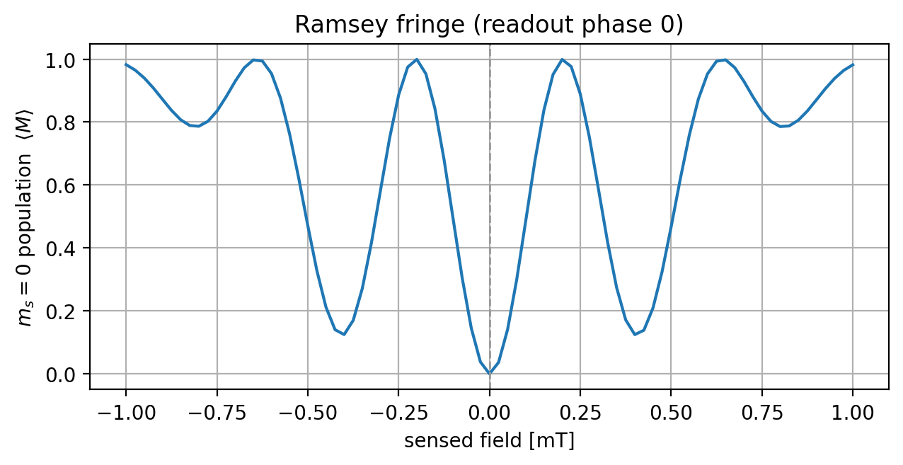
The fringe bears out the physics: \(B=0\) lands on an extremum, where the response is flat. The oscillation also shrinks toward the edges of the sweep — the field is on during the \(\pi/2\) pulses too, so at \(B=\pm1\) mT the Zeeman shift (\(\gamma_e B\approx28\) MHz) rivals the pulses’ own Rabi frequency (\(\approx8.3\) MHz), detuning them so they mis-rotate the spin. Neither affects what follows: slope detection operates at \(B=0\), and the recovered field is microtesla-scale, far below where this sets in.
Stage 2: reading it out — slope detection
The readout gives the \(m_s=0\) population \(p \equiv \langle M\rangle\), a probability in \([0,1]\). To
invert \(p \to B\) we need the response \(dp/dB\), and where we sit
on the fringe sets it. On the fringe above, \(B=0\) sits on an extremum, where the response is flat
(\(\delta p \approx 0\) to first order in \(B\)) — a blind spot. The fix is to rotate the readout
axis: taking readout_phase = pi/2 shifts the working point a quarter period, onto the steep
midpoint \(p_0 = 0.5\), where the response is largest and linear. Running the sensor there is
slope detection (Degen et al., “Quantum Sensing”, Secs. III.C,
V.E). The scan below confirms \(|dp/dB|\) is largest at
\(\pi/2\) and vanishes at the extrema, then reads off the working-point slope.
The working-point slope and effective sensing time
At the working point (readout phase \(\pi/2\)) the population traces a sine of the sensed field,
symmetric about \(p_0 = \tfrac12\) and steepest at \(B = 0\). Differentiating there gives the working-point slope
which packs all three ingredients of the response into one number: the gyromagnetic gain \(\gamma_e\),
the fringe contrast \(C\), and \(\tau_\text{eff}\), the effective sensing time — the interval
over which the field actually winds up phase. It comes out a little longer than wait, because the
field keeps tilting the spin during the two finite \(\pi/2\) pulses as well, not only during the free
evolution between them. Rather than assume it, we read it straight off the measured slope:
The printed value, \(\tau_\text{eff} \approx 88\) ns, duly sits between wait \(= 50\) ns and the full
sequence length \(110\) ns.
def slope_at(readout_phase, delta=1e-9):
    '''Response dp/dB at B=0 for a given readout phase (central finite difference of <M>).'''
    return (ramsey_signal(delta, readout_phase) - ramsey_signal(-delta, readout_phase)) / (2 * delta)

# Illustration: the response |dp/dB| and the working point p0 across readout phases. The response is
# largest exactly where p0 = 0.5 (readout phase pi/2) and vanishes at the fringe extrema.
readout_scan = np.linspace(0, np.pi, 19)
slope_scan = np.array([slope_at(phase) for phase in readout_scan])
p0_scan = np.array([ramsey_signal(0.0, phase) for phase in readout_scan])

fig, ax1 = plt.subplots(figsize=(6.5, 3.4))
ax1.plot(readout_scan, np.abs(slope_scan), 'o-', color='C0')
ax1.axvline(np.pi / 2, color='0.6', lw=1, ls='--')
ax1.set_xlabel('readout phase [rad]')
ax1.set_ylabel(r'response $|dp/dB|$   [1/T]', color='C0')
ax1.tick_params(axis='y', labelcolor='C0')
ax2 = ax1.twinx()
ax2.plot(readout_scan, p0_scan, 's--', color='C1', alpha=0.7)
ax2.set_ylabel(r'working point $p_0$', color='C1')
ax2.tick_params(axis='y', labelcolor='C1')
ax1.set_title(r'response is maximal at the $p_0=0.5$ working point ($\pi/2$)')
plt.tight_layout()
plt.show()

# Operate at the working point, readout phase pi/2.
p0 = ramsey_signal(0.0, np.pi / 2)
slope = slope_at(np.pi / 2)
tau_eff = abs(slope) / (np.pi * gyromagnetic_ratio)  # effective sensing time from |dp/dB| = pi*gamma*tau_eff*C
print(f'working point p0       = {p0:.4f}   (expect 0.5)')
print(f'response |dp/dB|       = {abs(slope):.0f} 1/T')
sequence_length = 2 * duration + wait  # full pi/2 - wait - pi/2 duration [us]
print(f'effective sensing time = {tau_eff * 1e3:.1f} ns   (between wait = {wait * 1e3:.0f} ns and the full sequence = {sequence_length * 1e3:.0f} ns: the field acts during the two pi/2 pulses too)')
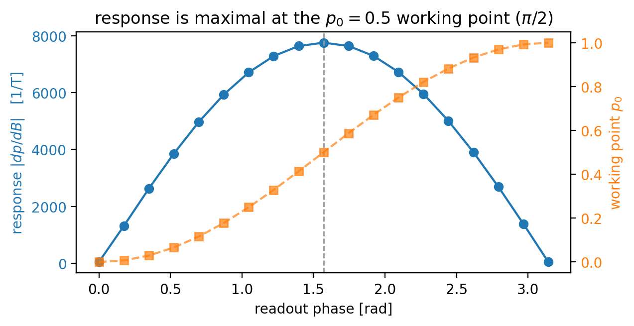
working point p0       = 0.5003   (expect 0.5)
response |dp/dB|       = 7765 1/T
effective sensing time = 88.2 ns   (between wait = 50 ns and the full sequence = 110 ns: the field acts during the two pi/2 pulses too)
The limit: how small a field can we resolve?
Two things set the smallest resolvable field: how strongly the field moves the readout (the slope we just measured) and how noisy each readout is. At the working point the response is linear, \(|dp/dB| = \pi\gamma_e\tau C\), and projection noise on \(p\), averaged over the measurement time, gives the shot-noise-limited sensitivity
with three factors, each from one step of the measurement: the transducer gain \(\gamma_e\) (field→phase), the sensing time \(\tau\) (phase accumulated), and the contrast \(C \in [0,1]\). Here \(C\) is an effective contrast that folds in two things which multiply: the Ramsey fringe visibility (how deep the interference fringe is, set by the pulses and dephasing) and the fluorescence readout contrast (how well the weak optical readout tells \(m_s{=}0\) from \(m_s{=}\pm1\) — only a few percent for a room-temperature NV, where the readout is photon-shot-noise-limited). Since \(\eta_B \propto 1/C\), the contrast is the factor you can fight for.
Where the formula comes from
Each shot ends in a projective readout, so the estimated population \(p\) carries irreducible quantum noise. At the working point \(p_0 = \tfrac12\) a single shot has the largest possible spread, \(\delta p = \sqrt{p_0(1-p_0)} = \tfrac12\), and averaging \(n_\text{shot}\) independent repetitions narrows it as
What the Ramsey sequence really estimates, though, is not \(p\) itself but the accumulated phase \(\phi = 2\pi\gamma_e B\,\tau\). Near the working point the fringe slope is \(|dp/d\phi| = C/2\), so the population noise becomes a phase uncertainty
— the standard interferometer limit: a full-contrast fringe (\(C = 1\)) resolves about one radian per shot, and averaging buys \(\sqrt{n_\text{shot}}\). Inverting \(\phi = 2\pi\gamma_e B\,\tau\) carries this back into a field uncertainty, \(\delta B = \delta\phi / (2\pi\gamma_e\,\tau)\). Finally, a fixed total time \(T\) buys \(n_\text{shot} = T/\tau\) shots, so \(\delta B\) falls as \(1/\sqrt{T}\); writing that as \(\delta B = \eta_B/\sqrt{T}\) and dropping the order-1 \(2\pi\) leaves the sensitivity
(The \(C\) in this derivation is the interferometric fringe visibility; the fluorescence readout contrast folds in on top, as noted above — see Taylor 2008; Barry 2020.)
What caps the sensing time. The response grows with \(\tau\), so you would take \(\tau \to \infty\) and resolve any field — except the fringe decoheres: past the coherence time \(T_2^*\) the contrast collapses, so the useful sensing time is capped at \(\tau \lesssim T_2^*\). Here the spin is ideal and \(C = 1\), so the fringe swings the full \(0 \to 1\):
def sensitivity(contrast):
    '''Shot-noise-limited sensitivity [T/sqrt(Hz)] gyromagnetic_ratio -> Hz/T, wait -> s.'''
    return 1.0 / (gyromagnetic_ratio * 1e6 * max(contrast, 1e-9) * np.sqrt(wait * 1e-6))

print(f'contrast C            = 1.0   (single ideal spin, full swing)')
print(f'ideal sensitivity eta = {sensitivity(1.0):.3e} T/sqrt(Hz) = {sensitivity(1.0) * 1e9:.1f} nT/sqrt(Hz)')
contrast C            = 1.0   (single ideal spin, full swing)
ideal sensitivity eta = 1.595e-07 T/sqrt(Hz) = 159.5 nT/sqrt(Hz)
Putting it to work: recovering an unknown field
The measurement now runs end to end. We treat the field as unknown: the analysis below uses only the measured signal, as a real measurement does, and compares against the true value at the end. With the instrument calibrated (\(p_0\) and the slope), a single measurement at the working point recovers the field by linear inversion, \(B_\text{est} = (p - p_0)/(dp/dB)\).
unknown_field = 8e-6  # T -- used only via the measured signal

p_measured = ramsey_signal(unknown_field, np.pi / 2)
estimated_field = (p_measured - p0) / slope

print(f'measured p         = {p_measured:.5f}')
print(f'estimated field    = {estimated_field * 1e6:.4f} uT')
print(f'true field         = {unknown_field * 1e6:.4f} uT')
print(f'relative error     = {abs(estimated_field - unknown_field) / abs(unknown_field):.2e}')
measured p         = 0.56223
estimated field    = 7.9789 uT
true field         = 8.0000 uT
relative error     = 2.64e-03
The recovery is essentially exact because this notebook is noiseless. In practice the three
factors behave very differently. \(\gamma_e\) is fixed by nature. The sensing time \(\tau\) is
capped by dephasing — grow it past the coherence time and the fringe washes out. That
coherence time is set by how spread-out the ensemble’s resonance frequencies are — the quantity
Part 2 introduces and quantifies (shot noise and \(T_2^*\) are modeled in
6_example_ramsey_with_quasistatic_noise.ipynb). That leaves
the contrast \(C\) as the factor you can actually fight for — and in a real device it is the
one under threat: an ensemble of spins with spread-out resonances loses contrast fast. Part 2
shows how the contrast collapses; Part 3 recovers it with an optimized pulse.
Part 2: The ensemble and the contrast
A single NV resolves maybe \(\sim\mu\text{T}/\sqrt{\text{Hz}}\); a real diamond magnetometer instead reads out many NVs at once — a macroscopic crystal holds \(10^9\)–\(10^{12}\) of them, and \(N\) spins together give a \(\sqrt{N}\) sensitivity boost (down to \(\text{fT}\)–\(\text{pT}/\sqrt{\text{Hz}}\)). It is tempting to get that \(N\) by simply packing the NVs denser, but density is self-defeating: denser spins broaden one another’s resonance, and that broadening is precisely what collapses the fringe contrast \(C\) (below). So the \(\sqrt{N}\) gain comes from a larger sensing volume, not a higher density — and there is an optimal density beyond which more NVs stop helping. Here we hold the per-spin picture and isolate that contrast collapse.
Why there's an optimal NV density
Raising the density pulls two ways at once:
more spins — \(N\) is the density times the sensing volume, and the signal-to-noise grows as \(\sqrt{N}\);
worse coherence — a denser NV (and nitrogen) bath widens the spread of resonance frequencies, \(\sigma \propto\) density. This is the same \(\sigma\) that shrinks the contrast \(C\) and the coherence time \(T_2^* \approx 1/(2\pi\sigma)\) studied here.
At a fixed volume the two roughly cancel: packing tighter gives more spins but each one is worse, so past an optimal density the added broadening eats the added spins and more NVs stop helping. The sensitivity therefore improves with the number of useful spins — which you grow with a larger crystal (more volume), not by squeezing harder. (A single NV is one spin in a vanishing volume, so it has no \(\sqrt{N}\) at all — that is why an ensemble beats it.)
This is where Part 3 comes in: recovering the contrast lost to broadening lets the ensemble tolerate a larger \(\sigma\) (a denser packing) before the signal collapses, so the optimal density shifts upward — more useful NVs in the same volume, and a better sensitivity.
Modelling the broadening
We model the broadening as a normally distributed static detuning of width \(\sigma\) (in MHz). This
\(\sigma\) is not a new parameter: it is the linewidth that set the \(T_2^*\) limit of Part 1, through
\(T_2^* \approx 1/(2\pi\sigma)\). So \(\sigma = 4\) MHz means \(T_2^* \approx 40\) ns — comparable to
the Ramsey wait, which is why the sensing time here is short. To sample the distribution, instead of using e.g. Monte Carlo, we take the weighted average of 11 different linewidth perturbation.
Two things then erode the contrast \(C\) as \(\sigma\) grows: (i) a rectangular \(\pi/2\) only rotates a resonant spin correctly — off-resonant spins mis-rotate; and (ii) during the free evolution the spread of static detunings winds the fringes out of step (the \(T_2^*\) dephasing). We scan \(\sigma\) up to \(\sim4\) MHz (about half the Rabi frequency \(\Omega \approx 8.3\) MHz), measuring \(C\) as the amplitude of the first harmonic of \(\langle M\rangle\) over three readout phases (illustrated just below), averaged over the Gaussian detuning distribution deterministically.
readout_phases = np.array([0.0, 2 * np.pi / 3, 4 * np.pi / 3])

def contrast_first_harmonic(signals, readout_phases):
    '''Fringe visibility C in [0,1] from the m_s=0 population <M> sampled at the given readout phases.
    The factor of 2 is because <M> = 1/2 (1 + C cos) swings by only C peak-to-peak, half the
    first-harmonic phasor amplitude.'''
    signals = np.asarray(signals)
    cos_component = (2 / len(signals)) * np.sum(signals * np.cos(readout_phases))
    sin_component = (2 / len(signals)) * np.sum(signals * np.sin(readout_phases))
    return float(2 * np.hypot(cos_component, sin_component))

# Average over the Gaussian inhomogeneous-detuning distribution deterministically, using Gauss-Hermite quadrature
gauss_nodes, gauss_weights = np.polynomial.hermite_e.hermegauss(11)
gauss_weights = gauss_weights / np.sqrt(2 * np.pi)  # standard-normal weights, sum to 1

def ensemble_population(append_ramsey, sigma, readout_phase, field=0.0):
    '''Ensemble-averaged m_s=0 population <M> for a detuning std sigma [MHz] and a sensed field [T].'''
    population = 0.0
    for node, weight in zip(gauss_nodes, gauss_weights):
        model.remove_all_pulses()
        append_ramsey(1.0, readout_phase)  # pi/2 - wait - pi/2 on MW_x
        end = model.driving_field('MW_x').last_pulse_end
        model.driving_field('DC_z').add_rectangle_pulse(amplitude=field + (sigma * node) / gyromagnetic_ratio,
                                                        frequency=0.,
                                                        phase=0.,
                                                        duration=end,
                                                        start=0.)
        result = model.simulate_time_evolution(n_eval=2,
                                               n_split=50,
                                               apply_noise=False)
        result.initial_state = model.productstate({'e': 0})
        population += weight * result.expectation_value('M',
                                                        t_idx=-1,
                                                        in_qubit_subspace=False)[0, 0].item()
    return population

def ramsey_contrast(append_ramsey, sigma):
    signals = [ensemble_population(append_ramsey, sigma, phase) for phase in readout_phases]
    return contrast_first_harmonic(signals, readout_phases)
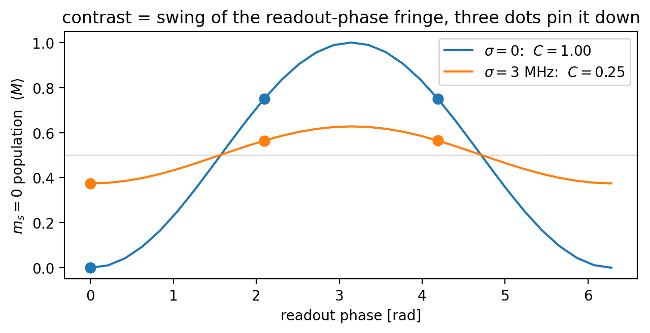
Why three readout phases? Sweeping the readout phase at \(B=0\) traces \(\langle M\rangle\) as a sinusoid of that phase, and its peak-to-peak swing is the contrast \(C\) — the amplitude of the first harmonic. A single sinusoid is fixed by three points, so sampling at \(\{0, 2\pi/3, 4\pi/3\}\) recovers \(C\) exactly. The plot overlays the readout-phase fringe at \(\sigma = 0\) (full swing) and \(\sigma = 3\) MHz (shrunk), with the three samples marked as dots.
phase_scan = np.linspace(0, 2 * np.pi, 31)
fringe_phase_narrow = np.array([ensemble_population(append_rectangular_ramsey, 0.0, ph) for ph in phase_scan])
fringe_phase_broad = np.array([ensemble_population(append_rectangular_ramsey, 3.0, ph) for ph in phase_scan])
samples_narrow = [ensemble_population(append_rectangular_ramsey, 0.0, ph) for ph in readout_phases]
samples_broad = [ensemble_population(append_rectangular_ramsey, 3.0, ph) for ph in readout_phases]

plt.figure(figsize=(6.5, 3.4))
plt.plot(phase_scan, fringe_phase_narrow, '-', color='C0',
         label=fr'$\sigma = 0$:  $C = {contrast_first_harmonic(samples_narrow, readout_phases):.2f}$')
plt.plot(phase_scan, fringe_phase_broad, '-', color='C1',
         label=fr'$\sigma = 3$ MHz:  $C = {contrast_first_harmonic(samples_broad, readout_phases):.2f}$')
plt.plot(readout_phases, samples_narrow, 'o', color='C0', markersize=7)
plt.plot(readout_phases, samples_broad, 'o', color='C1', markersize=7)
plt.axhline(0.5, color='0.85', lw=1, zorder=0)
plt.xlabel('readout phase [rad]')
plt.ylabel(r'$m_s{=}0$ population  $\langle M\rangle$')
plt.title('contrast = swing of the readout-phase fringe, three dots pin it down')
plt.legend()
plt.tight_layout()
plt.show()
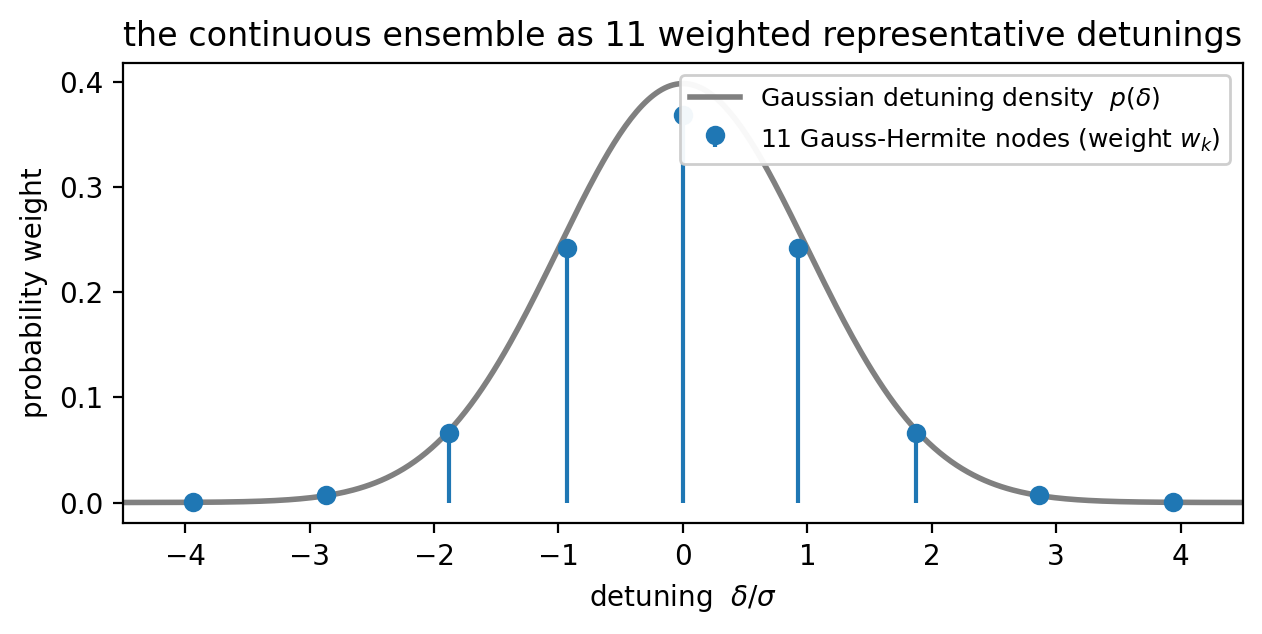
That deterministic average is an 11-point Gauss–Hermite quadrature: the continuous Gaussian ensemble is replaced by 11 representative detunings \(\delta_k = \sigma\,x_k\), each carrying a weight \(w_k\) (with \(\sum_k w_k = 1\)). The nodes concentrate where the Gaussian has its mass, so 11 points already give a machine-accurate average where random sampling would need thousands — and the curves come out reproducible, not shot-noise-limited.
x = np.linspace(-4.5, 4.5, 400)
plt.figure(figsize=(6.5, 3.3))
plt.plot(x, np.exp(-x**2 / 2) / np.sqrt(2 * np.pi), color='0.5', lw=2,
         label=r'Gaussian detuning density  $p(\delta)$')
plt.stem(gauss_nodes, gauss_weights, linefmt='C0-', markerfmt='C0o', basefmt=' ',
         label=r'11 Gauss-Hermite nodes (weight $w_k$)')
plt.xlim(-4.5, 4.5)
plt.xlabel(r'detuning  $\delta / \sigma$')
plt.ylabel('probability weight')
plt.title('the continuous ensemble as 11 weighted representative detunings')
plt.legend(loc='upper right', framealpha=0.95, fontsize=9)
plt.tight_layout()
plt.show()
Watching the fringe wash out
The quickest way to see the broadening bite is the Ramsey fringe itself. Sweeping the sensed field at readout phase 0 (as in Part 1) traces the fringe in \(\langle M\rangle\), and its peak-to-peak swing is the contrast \(C\). Overlaying the noiseless single-spin fringe from Part 1 with a representative ensemble (\(\sigma = 3\) MHz) under the rectangular pulse shows that swing collapse directly.
sigma_show = 3.0
fringe_fields = np.linspace(-1.0e-3, 1.0e-3, 31)  # +-1 mT

fringe_rectangular = np.array([ensemble_population(append_rectangular_ramsey, sigma_show, 0.0, field=field)
                               for field in fringe_fields])

plt.figure(figsize=(6.5, 3.4))
plt.plot(fields * 1e3, fringe_single, '-', color='C0',
         label='single spin (noiseless)')
plt.plot(fringe_fields * 1e3, fringe_rectangular, 'o-', markersize=3, color='C1',
         label=fr'ensemble, rectangular ($\sigma$ = {sigma_show} MHz, washed out)')
plt.axhline(0.5, color='0.85', lw=1, zorder=0)
plt.xlabel('sensed field [mT]')
plt.ylabel(r'$m_s{=}0$ population  $\langle M\rangle$')
plt.title('the ensemble washes the Ramsey fringe out')
plt.legend()
plt.grid(alpha=0.3)
plt.tight_layout()
plt.show()
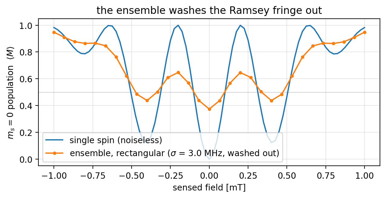
Quantifying the collapse
That single snapshot becomes a trend by scanning the linewidth \(\sigma\): at each \(\sigma\) we read off the contrast \(C\) (first harmonic over the three readout phases) and the sensitivity \(\eta = 1/(\gamma_e C\sqrt{\tau})\) it implies.
sigmas = np.array([0.0, 1.0, 2.0, 3.0, 4.0])  # up to ~ the Rabi frequency
contrast_rectangular = np.array([ramsey_contrast(append_rectangular_ramsey, s) for s in sigmas])
sensitivity_rectangular = np.array([sensitivity(c) for c in contrast_rectangular])

fig, axs = plt.subplots(1, 2, figsize=(11, 3.6))
axs[0].plot(sigmas, contrast_rectangular, 'o-', color='C0')
axs[0].set_xlabel(r'inhomogeneous linewidth $\sigma$ [MHz]')
axs[0].set_ylabel('Ramsey contrast $C$')
axs[0].set_ylim(0, 1.05)
axs[0].grid(alpha=0.3)
axs[1].semilogy(sigmas, sensitivity_rectangular, 'o-', color='C0')
axs[1].set_xlabel(r'inhomogeneous linewidth $\sigma$ [MHz]')
axs[1].set_ylabel(r'ideal sensitivity $\eta$ [T/$\sqrt{\mathrm{Hz}}$]')
axs[1].grid(alpha=0.3)
fig.suptitle(r'the rectangular pulse: contrast (and sensitivity) collapse as the linewidth $\sigma$ grows')
plt.tight_layout()
plt.show()
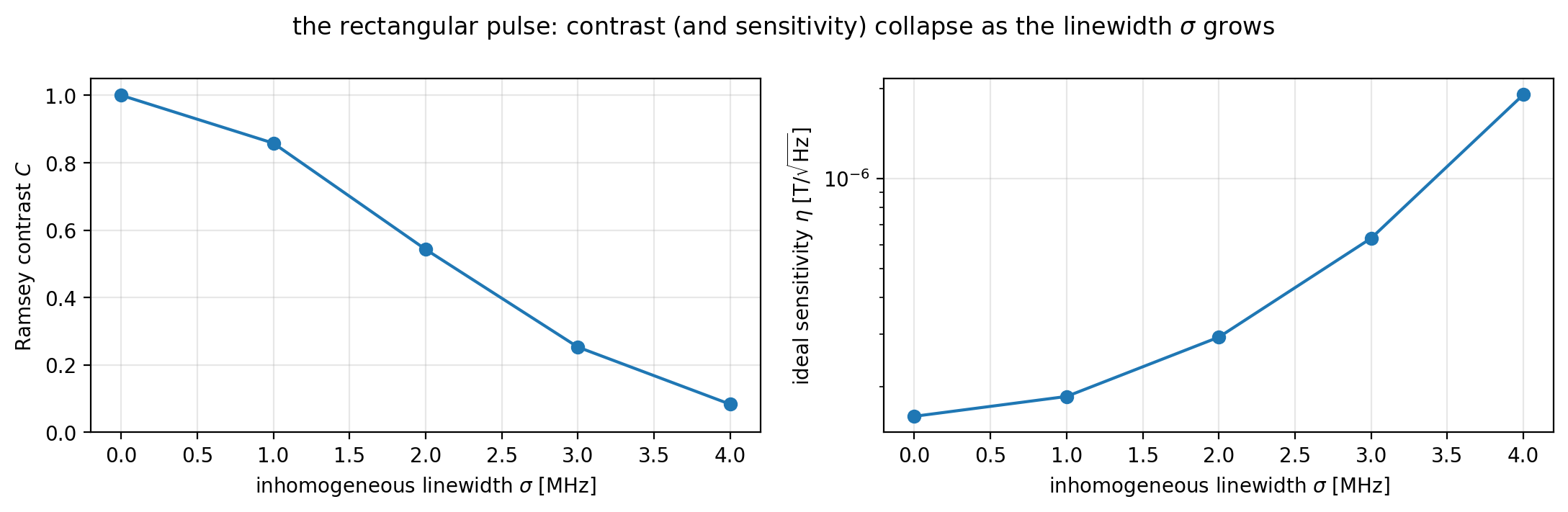
The contrast — and with it the sensitivity — falls off steadily as the linewidth \(\sigma\) grows. Crucially, the detuning spread is static (quasistatic / inhomogeneous), so it is refocusable: a pulse designed as part of the whole sequence can undo both the mis-rotation and the free-evolution dephasing, rather than just preparing a better superposition. Building that pulse is Part 3.
Part 3: Optimizing the pulse for robust sensitivity
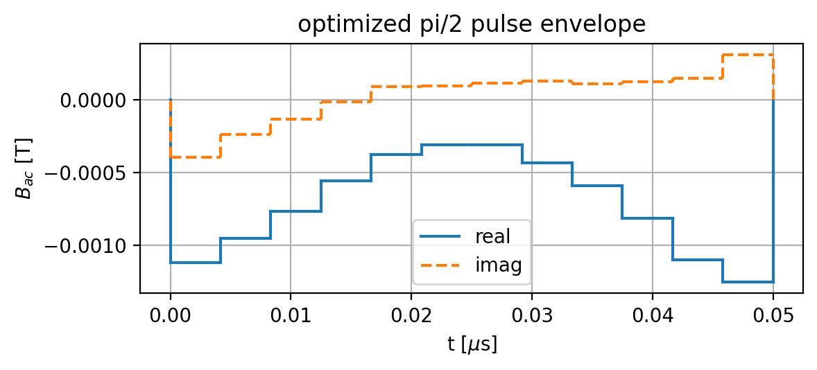
We replace the rectangular \(\pi/2\) with a piecewise-constant (GRAPE-style) pulse
(add_discrete_pulse, the two microwave quadratures) and let
Simphony’s autodiff shape it. The objective is the
sensing quantity itself — the ensemble sensitivity \(\eta\) — scored on the full Ramsey
interferometer (the same pulse used for preparation and readout), averaged over the inhomogeneous
detuning ensemble with the same deterministic Gauss–Hermite quadrature as Part 2 (so the
objective is exactly the sensitivity measured afterwards) and a small control-amplitude grid.
Running the optimization. Simphony differentiates all the way through the full Ramsey interferometer, so the optimizer improves the sensing figure of merit directly. Gradient-based optimization loops are compute-intensive, so — as is standard in optimal control — the optimization is run once, offline (a few tens of minutes); the resulting pulse is then loaded and evaluated with the NumPy backend.
Show the offline optimization code
import simphony
simphony.Config.set_platform('gpu')
simphony.Config.set_autodiff_mode(True)  # differentiable simulation
import jax.numpy as jnp
from jax import value_and_grad
from scipy.optimize import minimize

n_segments = 12
duration_opt = 0.05  # optimized pulse duration [us]
dt = duration_opt / n_segments
readout_phases = jnp.array([0.0, 2 * np.pi / 3, 4 * np.pi / 3])  # 3 readout phases -> true visibility
amplitude_grid = [0.9, 1.1]  # control-amplitude (Rabi) spread
sigma_train = 4.0  # inhomogeneous linewidth [MHz]

def ensemble_population(samples, scale, readout_phase):
    '''Deterministic Gauss-Hermite average of <M> over the detuning spread -- the same quadrature
    (gauss_nodes / gauss_weights) the Part 2 evaluation uses, so the objective is exactly the
    sensitivity we measure later, and the gradient stays smooth (no random-shot sampling).'''
    pulse = samples * scale
    population = 0.0
    for node, weight in zip(gauss_nodes, gauss_weights):
        model.remove_all_pulses()
        model.driving_field('MW_x').add_discrete_pulse(samples=pulse,
                                                       frequency=frequency,
                                                       dt=dt)
        model.driving_field('MW_x').add_wait(wait)
        model.driving_field('MW_x').add_discrete_pulse(samples=pulse * jnp.exp(1j * readout_phase),
                                                       frequency=frequency,
                                                       dt=dt)
        end = model.driving_field('MW_x').last_pulse_end
        model.driving_field('DC_z').add_rectangle_pulse(amplitude=(sigma_train * node) / gyromagnetic_ratio,
                                                        frequency=0.,
                                                        phase=0.,
                                                        duration=end,
                                                        start=0.)
        result = model.simulate_time_evolution(n_eval=2,
                                               n_split=50,
                                               apply_noise=False,
                                               verbose=False)
        result.initial_state = model.productstate({'e': 0})
        population = population + weight * result.expectation_value('M',
                                                                    t_idx=-1,
                                                                    in_qubit_subspace=False).ravel()[0]
    return population

def mean_sensitivity(params):  # the sensing figure of merit
    samples = params[:n_segments] + 1j * params[n_segments:]
    total = 0.0
    for scale in amplitude_grid:
        signals = jnp.array([ensemble_population(samples, scale, phase) for phase in readout_phases])
        cos_component = (2 / 3) * jnp.sum(signals * jnp.cos(readout_phases))
        sin_component = (2 / 3) * jnp.sum(signals * jnp.sin(readout_phases))
        contrast = jnp.clip(2 * jnp.hypot(cos_component, sin_component), 1e-3, None)  # <M> swings by C peak-to-peak
        total = total + 1.0 / (gyromagnetic_ratio * 1e6 * contrast * jnp.sqrt(wait * 1e-6))
    return total / len(amplitude_grid)

value_and_gradient = value_and_grad(mean_sensitivity)
def objective(x):
    value, gradient = value_and_gradient(jnp.array(x))
    return float(value), np.asarray(gradient, dtype=float)

seed_amplitude = model.rabi_amplitude_qubit(driving_field_name='MW_x',
                                            period_time=4 * duration_opt,
                                            spin_name='e')
np.random.seed(0)
initial = np.concatenate([np.full(n_segments, float(seed_amplitude)), np.zeros(n_segments)]) \
          + 0.05 * float(seed_amplitude) * np.random.randn(2 * n_segments)
peak = 6 * amplitude  # amplitude bound (power budget)

result = minimize(objective, initial, jac=True, method='L-BFGS-B',
                  bounds=[(-peak, peak)] * (2 * n_segments), options={'maxiter': 60})
optimized_params = result.x
The converged parameters from that offline run are stored below:
optimized_params = np.array([-0.001122743, -0.000954964, -0.000769573, -0.000559056, -0.000375531, -0.000312623, -0.00031127, -0.00043495, -0.000593487, -0.000817884, -0.001103305, -0.001253909, -0.000396127, -0.00023851, -0.000136765, -1.4079e-05, 9.1171e-05, 9.2421e-05, 0.000114065, 0.000128478, 0.000107912, 0.000121936, 0.000147232, 0.000307588])
n_segments = 12
duration_opt = 0.05  # optimized pulse duration [us]
dt = duration_opt / n_segments
optimized_samples = optimized_params[:n_segments] + 1j * optimized_params[n_segments:]

def append_optimized_ramsey(scale, readout_phase):
    pulse = optimized_samples * scale
    model.driving_field('MW_x').add_discrete_pulse(samples=pulse,
                                                   frequency=frequency,
                                                   dt=dt)
    model.driving_field('MW_x').add_wait(wait)
    model.driving_field('MW_x').add_discrete_pulse(samples=pulse * np.exp(1j * readout_phase),
                                                   frequency=frequency,
                                                   dt=dt)

model.remove_all_pulses()
model.driving_field('MW_x').add_discrete_pulse(samples=optimized_samples,
                                               frequency=frequency,
                                               dt=dt)
fig, ax = plt.subplots(figsize=(6, 2.8))
model.driving_field('MW_x').plot_pulses(function='complex_envelope', ax=ax)
ax.set_title('optimized pi/2 pulse envelope')
plt.tight_layout()
plt.show()
Result: sensitivity that survives the ensemble
The clearest view is the Ramsey fringe itself. On the same sensed-field sweep and the same ensemble (\(\sigma = 3\) MHz) as Part 2, we add the optimized-pulse fringe to the noiseless single spin and the washed-out rectangular ensemble. It stays crisp — that recovered visibility is exactly the recovered sensitivity.
fringe_optimized = np.array([ensemble_population(append_optimized_ramsey, sigma_show, 0.0, field=field)
                             for field in fringe_fields])

plt.figure(figsize=(6.5, 3.4))
plt.plot(fields * 1e3, fringe_single, '-', color='C0', label='single spin (noiseless)')
plt.plot(fringe_fields * 1e3, fringe_rectangular, 'o-', markersize=3, color='C1', label='ensemble, rectangular (washed out)')
plt.plot(fringe_fields * 1e3, fringe_optimized, 's-', markersize=3, color='C2', label='ensemble, optimized (crisp)')
plt.axhline(0.5, color='0.85', lw=1, zorder=0)
plt.xlabel('sensed field [mT]')
plt.ylabel(r'$m_s{=}0$ population  $\langle M\rangle$')
plt.title(fr'the optimized pulse restores the fringe at $\sigma$ = {sigma_show} MHz')
plt.legend()
plt.tight_layout()
plt.show()
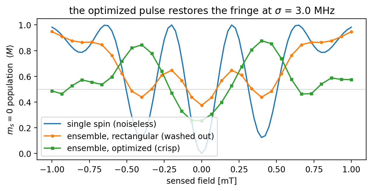
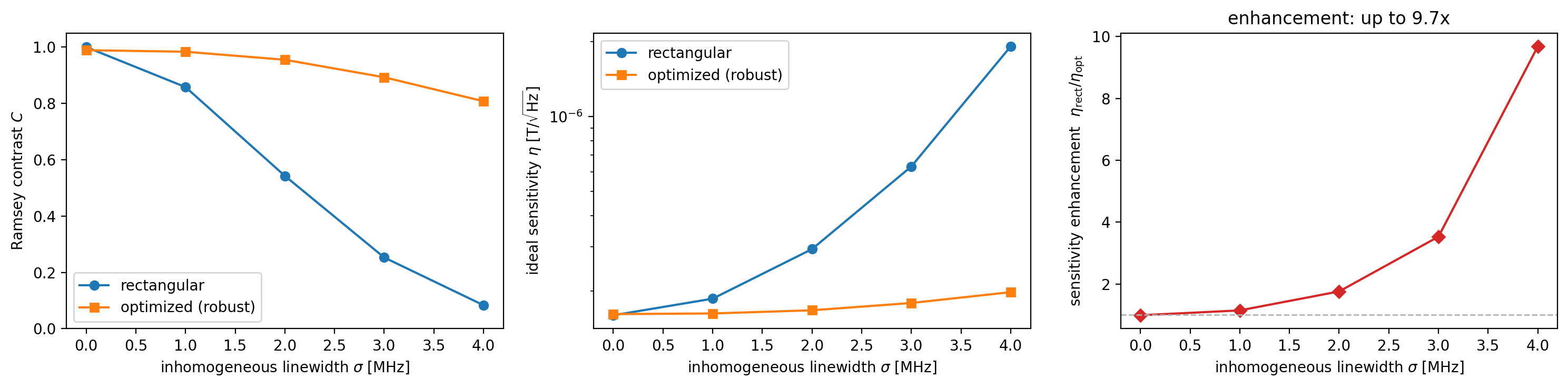
The gain across the linewidth
Sweeping the inhomogeneous linewidth \(\sigma\) turns that single snapshot into a trend, comparing the two pulses on equal footing — the full two-pulse Ramsey interferometer, same ensemble.
This is the same comparison Jauch et al. make experimentally. When the microwave drive is homogeneous — every spin seeing the same Rabi frequency — optimal control barely beats a rectangular \(\pi/2\) (\(\sim\!1.6\times\)): a hard pulse is already close to optimal. Under a realistic inhomogeneous drive, where the Rabi strength varies across the ensemble, the rectangular pulse mis-rotates the off-resonant spins much more, so the relative benefit of optimal control grows (\(\sim\!3\times\) in their setup) — the more inhomogeneous the drive, the more it helps. Our \(\sigma\)-scan is the same story along a different axis: they vary the microwave-field homogeneity, we vary the detuning linewidth \(\sigma\). The enhancement below is close to \(1\) at \(\sigma = 0\) and grows with \(\sigma\); the absolute numbers differ, but the trend — optimal control helping more as the inhomogeneity it fights grows — carries over.
contrast_optimized = np.array([ramsey_contrast(append_optimized_ramsey, s) for s in sigmas])
sensitivity_optimized = np.array([sensitivity(c) for c in contrast_optimized])
enhancement = sensitivity_rectangular / sensitivity_optimized

fig, axs = plt.subplots(1, 3, figsize=(15, 3.8))
axs[0].plot(sigmas, contrast_rectangular, 'o-', label='rectangular')
axs[0].plot(sigmas, contrast_optimized, 's-', label='optimized (robust)')
axs[0].set_xlabel(r'inhomogeneous linewidth $\sigma$ [MHz]')
axs[0].set_ylabel('Ramsey contrast $C$')
axs[0].set_ylim(0, 1.05)
axs[0].legend()

axs[1].semilogy(sigmas, sensitivity_rectangular, 'o-', label='rectangular')
axs[1].semilogy(sigmas, sensitivity_optimized, 's-', label='optimized (robust)')
axs[1].set_xlabel(r'inhomogeneous linewidth $\sigma$ [MHz]')
axs[1].set_ylabel(r'ideal sensitivity $\eta$ [T/$\sqrt{\mathrm{Hz}}$]')
axs[1].legend()

axs[2].plot(sigmas, enhancement, 'D-', color='C3')
axs[2].axhline(1.0, color='0.7', lw=1, ls='--')
axs[2].set_xlabel(r'inhomogeneous linewidth $\sigma$ [MHz]')
axs[2].set_ylabel(r'sensitivity enhancement  $\eta_\mathrm{rect}/\eta_\mathrm{opt}$')
axs[2].set_title(f'enhancement: up to {np.max(enhancement):.1f}x')

plt.tight_layout()
plt.show()
Summary and caveats
Part 1 established DC magnetometry with a single NV spin: a Ramsey sequence turns a field into a phase and then a population, slope detection reads it out linearly at the maximum-slope working point, and the sensitivity is \(\eta_B = 1/(\gamma_e C\sqrt{\tau})\) — set by the transducer gain \(\gamma_e\), the sensing time \(\tau\), and the fringe contrast \(C\).
Part 2 showed what an ensemble does to that measurement: inhomogeneous broadening (a static detuning spread \(\sigma\), the same \(T_2^*\approx1/(2\pi\sigma)\) limit as Part 1) both mis-rotates off-resonant spins under a rectangular \(\pi/2\) and dephases the fringe during free evolution, so the contrast \(C\) — and, via \(\eta \propto 1/C\), the sensitivity — collapses as \(\sigma\) grows.
Part 3 optimized the sensing figure of merit itself — not an abstract gate fidelity — by differentiating the full Ramsey interferometer through Simphony. Because the broadening is static (quasistatic / inhomogeneous), it is refocusable: a single pulse pair optimized over the whole sequence recovers the contrast lost to both mis-rotation and free-evolution dephasing, improving the ensemble sensitivity several-fold at large \(\sigma\) — the same qualitative trend Jauch et al. measure experimentally, where optimal control gains more as the microwave field becomes less homogeneous.
Caveats. The optimization targets both the detuning spread and (via a \(\pm10\%\)
amplitude_grid) the control-amplitude (Rabi) inhomogeneity — the drive strength varies across a real wide-field ensemble. Widening those training windows trades one robustness for the other. Piecewise-constant pulses are used in this strong-drive, short-\(\tau\) regime; smooth, bandwidth-limited pulses (via finer segments orrise_time/fall_time) are a direct extension. What this cannot fix is dynamic decoherence (\(T_2\), from fluctuating rather than static fields): no fixed pulse pair refocuses it, and it ultimately caps \(\tau\) — that regime needs dynamical decoupling and the noise machinery of6_example_ramsey_with_quasistatic_noise.ipynb.