The single-sine-wave method
Simphony has a dedicated method for constant-envelope, single-frequency (“single sine wave”)
pulses: instead of integrating the full pulse duration, it simulates just one period \(T\) of
the drive on n_split uniform sub-steps, and reconstructs the full-segment propagator by matrix
power,
This notebook is about the method itself: why the reconstruction is valid, exactly when Simphony
is allowed to use it (and what happens silently when it isn’t), how much speed it actually buys,
and how to build trust in it before relying on it for long pulses — including its
time_grid_jitter-related pitfall and fix, folded in below so this notebook is the single
self-contained reference for the method (see the “Time-grid jitter” section).
Import the packages
import time

import numpy as np
import matplotlib.pyplot as plt

import simphony

simphony.Config.set_platform('cpu')
simphony.Config.set_matplotlib_format('retina')
Model and pulse
We use a \(^{14}\)N-containing NV center and drive the nitrogen spin with a resonant NMR pulse on
RF_x — a constant-envelope, single-frequency drive, exactly the case the single-sine-wave
method targets. We calibrate a \(\pi/2\) pulse of duration \(10\,\mu\text{s}\) first, to see what
the method does on a typical case, then reuse the same frequency and carrier period T for the
rest of the notebook with pulses of other durations.
model = simphony.default_nv_model(nitrogen_isotope=14, static_field_strength=0.5)

angle = np.pi / 2
frequency = model.splitting_qubit('N', rest_quantum_nums={'e': 0})
T = 1 / abs(frequency)
print(f'carrier frequency = {frequency:.4f} MHz, carrier period T = {T:.4f} us')

duration = 10.0  # us
period_time = 2 * np.pi * duration / angle
amplitude = model.rabi_amplitude_qubit(driving_field_name='RF_x',
                                       period_time=period_time,
                                       spin_name='N',
                                       rest_quantum_nums={'e': 0})
model.driving_field('RF_x').add_rectangle_pulse(amplitude=amplitude,
                                                 frequency=frequency,
                                                 phase=0.0,
                                                 duration=duration)

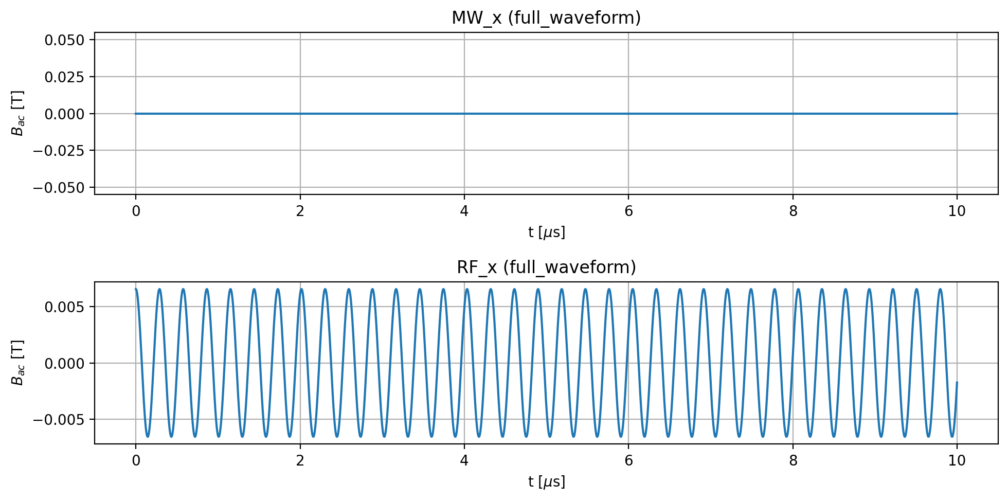
model.plot_driving_fields(function='full_waveform')
carrier frequency = -3.4707 MHz, carrier period T = 0.2881 us
Why one period is enough
The single-sine-wave method applies whenever the driving Hamiltonian \(H(t)\) is periodic with period \(T = 1/f\) (the drive’s carrier period), i.e. \(H(t + T) = H(t)\) throughout the pulse. Time evolution under any time-dependent Hamiltonian satisfies, independent of periodicity, the composition property
i.e. propagating to a later time factors through any intermediate time. Periodicity of \(H\) adds one more fact, shift invariance:
because the equation of motion at times shifted by a whole period is identical to the unshifted one. Combining the two: write \(nT + \tau\) for \(n\) full periods plus a remainder \(0 \le \tau < T\). Using composition to split off the last period, then shift invariance to identify it with the very first period,
Applying composition and shift invariance repeatedly to \(U(nT, 0)\) in the same way gives \(U(nT, 0) = [U(T, 0)]^n\), so
Only \(U(\tau, 0)\) for \(\tau \in [0, T)\) and the single-period propagator \(U(T, 0)\) need to be simulated numerically; the rest of an arbitrarily long pulse is reconstructed by matrix power, an \(\mathcal{O}(\log n)\) operation via repeated squaring, instead of simulating every period from scratch.
This is purely an internal computational shortcut: the evaluation times you actually request
(n_eval points spread across the whole pulse, via simulate_time_evolution) are still returned
at exactly those same points, uniformly across the full duration — each requested time is
projected onto its equivalent phase within the one simulated period, and the corresponding period
count \(n\) is tracked and applied via the matrix power. Nothing about the method’s output changes;
only how it gets computed does.
This also stays compatible with Simphony’s current noise model, quasistatic noise: a noise realization is a fixed, randomly-drawn shift added to the Hamiltonian for the whole duration of one shot, not something that varies in time within that shot. Adding a time-independent term to a periodic \(H(t)\) doesn’t break its periodicity — it’s still periodic with the same \(T\), just shifted — so the same derivation goes through per shot, with \(U(T, 0)\) (and hence the whole reconstruction) reflecting that shot’s particular noise realization.
Eligibility conditions
Simphony doesn’t use the single-sine-wave method whenever it could in principle — it checks three concrete conditions every time a segment is simulated:
exactly one nonzero drive frequency,
a constant envelope for the whole segment,
at least one full period fits in the segment.
If any of these fails, Simphony silently falls back to simulation_method='basic' for that
segment — no warning, no error, just a slower (but still correct) simulation. The clearest way
to break the third condition is a pulse shorter than one carrier period:
model.remove_all_pulses()
period_time = 2 * np.pi * (0.5 * T) / angle
amplitude = model.rabi_amplitude_qubit(driving_field_name='RF_x',
                                       period_time=period_time,
                                       spin_name='N',
                                       rest_quantum_nums={'e': 0})
model.driving_field('RF_x').add_rectangle_pulse(amplitude=amplitude,
                                                 frequency=frequency,
                                                 phase=0.0,
                                                 duration=0.5 * T)

result = model.simulate_time_evolution(n_eval=2, n_split=250, verbose=True)
start = 0.0
end = 0.1440626239025144
solver_method = numpy_expm
number of simulated driving terms = 1
number of simulated noise terms = 0
---------------------------------------------------------------------------
simulate time segment [0.000, 0.144] with step size 0.001153 (type: basic)
As expected, the segment falls back to type: basic. A rise/fall time (breaking the constant
envelope) is more subtle: Simphony automatically splits the pulse into rise / constant / fall
sub-segments, so only the ramps fall back to basic while the constant middle keeps using
single_sine_wave:
model.remove_all_pulses()
period_time = 2 * np.pi * duration / angle
amplitude = model.rabi_amplitude_qubit(driving_field_name='RF_x',
                                       period_time=period_time,
                                       spin_name='N',
                                       rest_quantum_nums={'e': 0})
model.driving_field('RF_x').add_rectangle_pulse(amplitude=amplitude,
                                                 frequency=frequency,
                                                 phase=0.0,
                                                 duration=duration,
                                                 rise_time=1.0,
                                                 fall_time=1.0)

result = model.simulate_time_evolution(n_eval=2, n_split=250, verbose=True)
start = 0.0
end = 10.0
solver_method = numpy_expm
number of simulated driving terms = 1
number of simulated noise terms = 0
---------------------------------------------------------------------------
simulate time segment [0.00, 1.00] with step size 0.001153 (type: basic)
simulate time segment [1.00, 9.00] with step size 0.001153 (type: single_sine_wave)
simulate time segment [9.00, 10.00] with step size 0.001153 (type: basic)
Performance comparison
We compare wall-clock time for simulation_method='basic' vs. 'single_sine_wave' on the same
pulse, at a fixed per-period resolution (n_split_per_period steps per carrier period), as the
pulse duration grows from 10 to 30 carrier periods. For 'basic', matching that resolution means
n_split has to grow with the number of periods (it discretizes the whole duration); for
'single_sine_wave', n_split only ever covers a single period, so it stays fixed regardless of
how many periods the pulse spans.
n_split_per_period = 20
n_periods_list = [10, 20, 30]

times_basic = []
times_sine = []
for n_periods in n_periods_list:
    duration_sweep = n_periods * T

    model.remove_all_pulses()
    period_time = 2 * np.pi * duration_sweep / angle
    amplitude = model.rabi_amplitude_qubit(driving_field_name='RF_x',
                                           period_time=period_time,
                                           spin_name='N',
                                           rest_quantum_nums={'e': 0})
    model.driving_field('RF_x').add_rectangle_pulse(amplitude=amplitude,
                                                     frequency=frequency,
                                                     phase=0.0,
                                                     duration=duration_sweep)

    n_split_basic = n_periods * n_split_per_period

    t0 = time.perf_counter()
    model.simulate_time_evolution(n_eval=2, n_split=n_split_basic, simulation_method='basic')
    times_basic.append(time.perf_counter() - t0)

    t0 = time.perf_counter()
    model.simulate_time_evolution(n_eval=2, n_split=n_split_per_period, simulation_method='single_sine_wave')
    times_sine.append(time.perf_counter() - t0)

    print(f'n_periods={n_periods:>3d}  n_split_basic={n_split_basic:>5d}  '
          f't_basic={times_basic[-1]:7.3f} s  t_single_sine_wave={times_sine[-1]:7.4f} s')
n_periods= 10  n_split_basic=  200  t_basic=  0.762 s  t_single_sine_wave= 0.0104 s
n_periods= 20  n_split_basic=  400  t_basic=  2.875 s  t_single_sine_wave= 0.0143 s
n_periods= 30  n_split_basic=  600  t_basic=  9.026 s  t_single_sine_wave= 0.0156 s
fig, ax = plt.subplots(figsize=(6, 4), constrained_layout=True)
ax.plot(n_periods_list, times_basic, 'o-', label='basic')
ax.plot(n_periods_list, times_sine, 'o-', label='single_sine_wave')
ax.set_yscale('log')
ax.set_xlabel('pulse duration (number of carrier periods)')
ax.set_ylabel('wall-clock time (s)')
ax.set_title('same per-period resolution, growing pulse duration')
ax.grid(True, which='both', linestyle=':')
ax.legend()
plt.show()
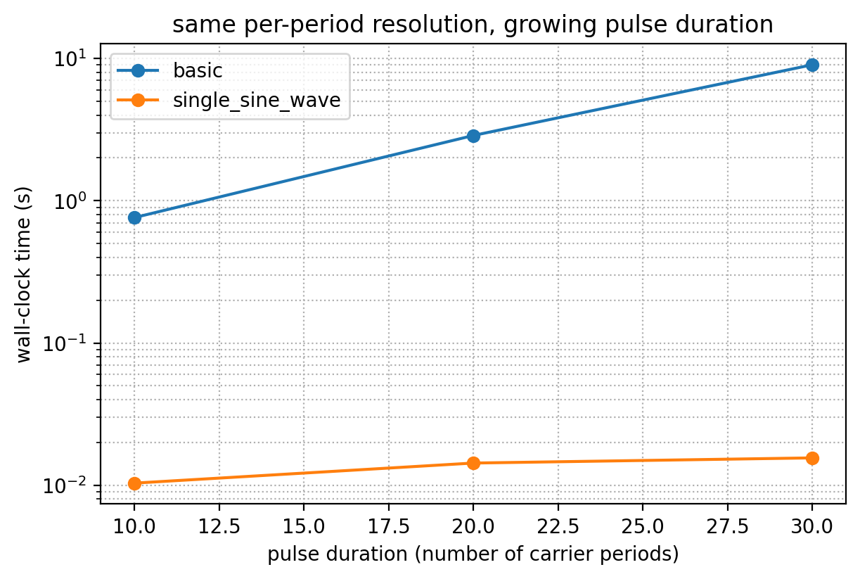
At matched resolution, 'basic'’s cost grows sharply with the pulse duration (and worse than
linearly here, since the per-step Python-loop overhead of 'basic' also scales with the number of
steps), while 'single_sine_wave' stays close to flat: it always only ever simulates one period,
no matter how many times that period repeats.
Correctness cross-check
Before trusting the single-sine-wave method on pulses long enough that 'basic' is impractical,
it’s worth directly checking the two methods agree on a case where 'basic' is still affordable
at high resolution.
duration_check = 5 * T

model.remove_all_pulses()
period_time = 2 * np.pi * duration_check / angle
amplitude = model.rabi_amplitude_qubit(driving_field_name='RF_x',
                                       period_time=period_time,
                                       spin_name='N',
                                       rest_quantum_nums={'e': 0})
model.driving_field('RF_x').add_rectangle_pulse(amplitude=amplitude,
                                                 frequency=frequency,
                                                 phase=0.0,
                                                 duration=duration_check)

n_split_check = 200

result_basic = model.simulate_time_evolution(n_eval=2, n_split=n_split_check, simulation_method='basic')
result_sine = model.simulate_time_evolution(n_eval=2, n_split=n_split_check, simulation_method='single_sine_wave')

U_basic = result_basic.time_evol_operator.matrix(t_idx=-1)[0, 0]
U_sine = result_sine.time_evol_operator.matrix(t_idx=-1)[0, 0]

infidelity = 1 - simphony.utils.average_gate_fidelity_from_unitaries(U_basic, U_sine)
print(f'infidelity between basic and single_sine_wave: {infidelity:.3e}')
infidelity between basic and single_sine_wave: 3.141e-13
The two methods agree to within numerical precision, confirming the matrix-power reconstruction is correct, not just fast.
Time-grid jitter
The single-sine-wave method has one subtle failure mode worth knowing about: because it reuses the
exact same uniform sample points within every period, certain n_split values put those sample
points into a numerical “resonance” with the sine’s own structure. The resulting error in the
single-cycle propagator \(U(T)\) isn’t small and random — it’s systematic, and it gets amplified
by the \(n\)-th power reconstruction. Instead of the infidelity smoothly decreasing as n_split
grows, it spikes sharply at certain resonant values and dips at others.
Prediction: sweeping n_split on a fixed uniform grid should show sharp, non-monotonic,
periodically-recurring spikes in \(|1 - F(U, U_{\mathrm{ref}})|\). Randomly perturbing the interior
sub-step boundaries a little (time_grid_jitter) should break the exact phase alignment behind
those spikes, replacing the resonant sawtooth pattern with a flat, jitter-limited noise floor. We
verify both predictions below.
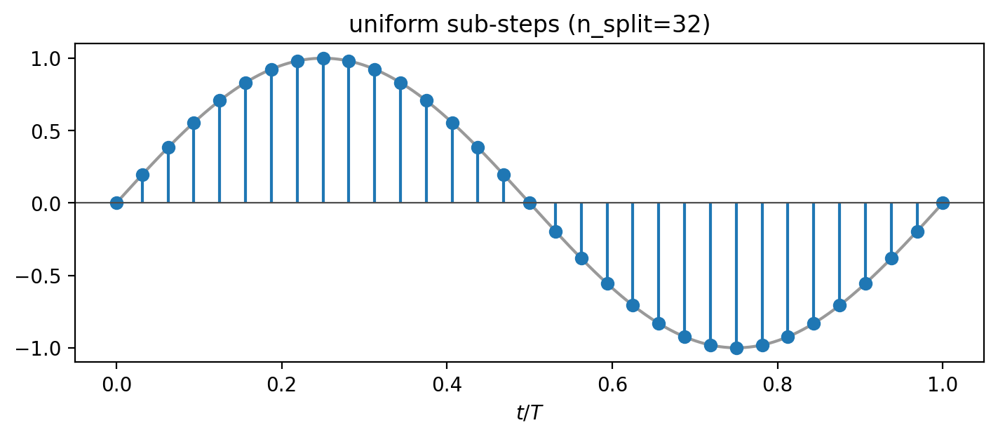
As a concrete picture of what “n_split uniform sub-steps within one period” means, here is
how n_split=32 divides a single sine period:
n_illustration = 32
t_illustration = np.linspace(0.0, 1.0, 1000)
wave_illustration = np.sin(2 * np.pi * t_illustration)
uniform_bounds = np.linspace(0.0, 1.0, n_illustration + 1)
uniform_values = np.sin(2 * np.pi * uniform_bounds)

fig, ax = plt.subplots(figsize=(7, 3), constrained_layout=True)
ax.plot(t_illustration, wave_illustration, color='0.6')
ax.vlines(uniform_bounds, 0, uniform_values, color='tab:blue')
ax.plot(uniform_bounds, uniform_values, 'o', color='tab:blue')
ax.axhline(0, color='0.3', linewidth=0.8)
ax.set_title(f'uniform sub-steps (n_split={n_illustration})')
ax.set_xlabel(r'$t / T$')
plt.show()
Now back to the actual pulse. We restore the original \(10\,\mu\text{s}\) pulse and use a very
fine fixed grid (n_split=100001) as a ground-truth propagator \(U_{\mathrm{ref}}\) to compare
against.
model.remove_all_pulses()
period_time = 2 * np.pi * duration / angle
amplitude = model.rabi_amplitude_qubit(driving_field_name='RF_x',
                                       period_time=period_time,
                                       spin_name='N',
                                       rest_quantum_nums={'e': 0})
model.driving_field('RF_x').add_rectangle_pulse(amplitude=amplitude,
                                                 frequency=frequency,
                                                 phase=0.0,
                                                 duration=duration)

result_ref = model.simulate_time_evolution(n_eval=2, n_split=100001, verbose=True)
U_ref = result_ref.time_evol_operator.matrix(t_idx=-1)[0, 0]
start = 0.0
end = 10.0
solver_method = numpy_expm
number of simulated driving terms = 1
number of simulated noise terms = 0
---------------------------------------------------------------------------
simulate time segment [0.0, 10.0] with step size 2.881e-06 (type: single_sine_wave)
We sweep n_split over a moderate range and compare each resulting propagator to
\(U_{\mathrm{ref}}\). Per the prediction above, we expect sharp, non-monotonic spikes rather than
smooth convergence.
n_splits = np.arange(2, 502, 1)

Us_fix = []
for idx, n_split in enumerate(n_splits):
    result = model.simulate_time_evolution(n_eval=2, n_split=n_split)
    Us_fix.append(result.time_evol_operator.matrix(t_idx=-1)[0, 0])
    if idx % 50 == 0:
        print(f'{idx}/{len(n_splits)}', end=' ')
print('done')
0/500 50/500 100/500 150/500 200/500 250/500 300/500 350/500 400/500 450/500 done
infids_fix = np.array([1 - simphony.utils.average_gate_fidelity_from_unitaries(U, U_ref) for U in Us_fix])

fig, ax = plt.subplots(figsize=(6, 4), constrained_layout=True)
ax.plot(n_splits, np.abs(infids_fix), '.-')
ax.set_yscale('log')
ax.set_xlabel('n_split')
ax.set_ylabel('infidelity')
ax.set_title(r'fixed grid: $|1 - F(U, U_{\mathrm{ref}})|$')
ax.grid(True, which='both', linestyle=':')
plt.show()
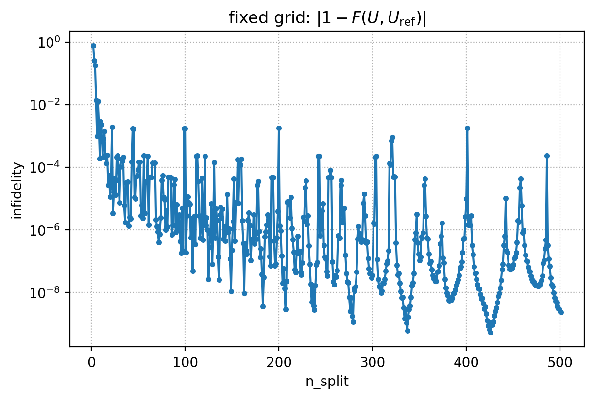
As predicted, the fixed-grid infidelity does not decrease monotonically with n_split —
it has sharp, periodically-recurring resonant spikes (roughly every 100 steps here) where the
sample points happen to line up unfavorably with the sine drive. Between spikes, though, some
“lucky” n_split values land the sample points so favorably that the error dips as low as
\(10^{-8}\) — far below the generic discretization error for that step count.
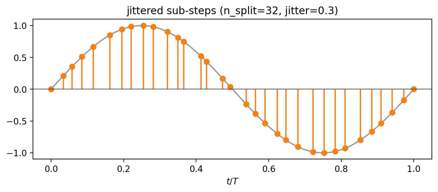
Now we repeat the same sweep with time_grid_jitter enabled, which randomly perturbs the interior
sub-step boundaries within each interval (interval endpoints are unaffected) by up to
jitter / n_split of the interval width. This should break the resonance and give a flat noise
floor instead. Here is the same single-period illustration with time_grid_jitter=0.3: the
interior boundaries move around, but the two endpoints of the period stay fixed:
jitter_illustration = 0.3
rng_illustration = np.random.default_rng(0)

# Same jitter rule as `compute_time_grid`: perturb interior boundaries by up to jitter / n_split of the interval width; endpoints stay fixed.
jittered_bounds = uniform_bounds.copy()
jittered_bounds[1:-1] += (rng_illustration.random(n_illustration - 1) * 2 - 1) * jitter_illustration / n_illustration
jittered_values = np.sin(2 * np.pi * jittered_bounds)

fig, ax = plt.subplots(figsize=(7, 3), constrained_layout=True)
ax.plot(t_illustration, wave_illustration, color='0.6')
ax.vlines(jittered_bounds, 0, jittered_values, color='tab:orange')
ax.plot(jittered_bounds, jittered_values, 'o', color='tab:orange')
ax.axhline(0, color='0.3', linewidth=0.8)
ax.set_title(f'jittered sub-steps (n_split={n_illustration}, jitter={jitter_illustration})')
ax.set_xlabel(r'$t / T$')
plt.show()
Us_jitter = []
for idx, n_split in enumerate(n_splits):
    result = model.simulate_time_evolution(n_eval=2, n_split=n_split, time_grid_jitter=0.3)
    Us_jitter.append(result.time_evol_operator.matrix(t_idx=-1)[0, 0])
    if idx % 50 == 0:
        print(f'{idx}/{len(n_splits)}', end=' ')
print('done')
0/500 50/500 100/500 150/500 200/500 250/500 300/500 350/500 400/500 450/500 done
infids_jitter = np.array([1 - simphony.utils.average_gate_fidelity_from_unitaries(U, U_ref) for U in Us_jitter])

fig, ax = plt.subplots(figsize=(6, 4), constrained_layout=True)
ax.plot(n_splits, np.abs(infids_fix), '.-', label='fixed', alpha=0.6)
ax.plot(n_splits, np.abs(infids_jitter), '.-', label='jittered (0.3)')
ax.set_yscale('log')
ax.set_xlabel('n_split')
ax.set_ylabel('infidelity')
ax.set_title(r'fixed vs. jittered grid: $|1 - F(U, U_{\mathrm{ref}})|$')
ax.grid(True, which='both', linestyle=':')
ax.legend()
plt.show()
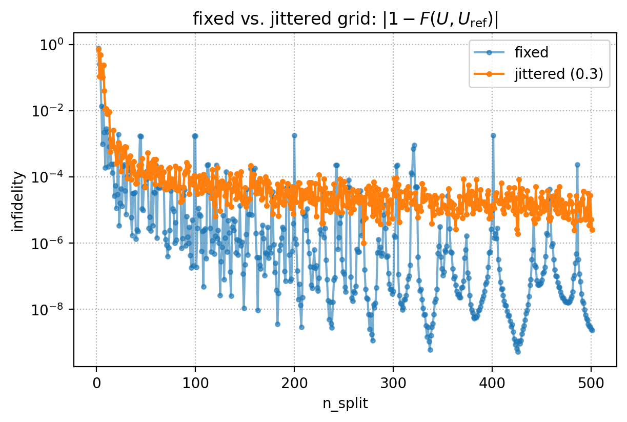
Confirmed, with a caveat: with jitter enabled, the periodic resonant spikes disappear entirely
— the sub-step boundaries no longer line up the same way on every period, so there’s no more
n_split value where the error catastrophically jumps back up. But the curve isn’t simply
“smoother and lower”: it settles into a flat, jitter-amplitude-limited noise floor around
\(10^{-4}\)–\(10^{-5}\), well above the fixed grid’s best “lucky” troughs (down to \(10^{-8}\)).
Jitter trades away both the fixed grid’s worst-case spikes and its best-case lucky dips for a
bounded, predictable error level.
simulate_time_evolution’s default n_split is 250. If a given pulse’s parameters happen to
place a resonant spike right at n_split=250, the default settings silently produce an inaccurate
result — nothing about the run itself signals this; you’d only notice by separately checking
convergence as a function of n_split, as we did above. Enabling time_grid_jitter removes the
need to hunt for a “safe” n_split by hand: jitter breaks the resonance, so even at the default
n_split=250 you reliably land on the generic, jitter-limited error level
(\(10^{-4}\)–\(10^{-5}\)) instead of risking an unlucky hit on a spike. The price is a slightly
higher typical error; the benefit is that no particular n_split value can be silently wrong.
Conclusion
The single-sine-wave method turns an \(\mathcal{O}(n)\) integration (one full period’s worth of
steps, repeated \(n\) times) into an \(\mathcal{O}(\log n)\) matrix-power reconstruction, which is why
its cost barely grows with pulse duration while 'basic'’s does, while still agreeing with
'basic' to within numerical precision. Simphony picks it automatically whenever a segment has a
single nonzero drive frequency, a constant envelope, and is at least one carrier period long
— and falls back to 'basic' silently otherwise, so it’s worth checking verbose=True
output if a simulation seems slower than expected. Its one real pitfall is the n_split resonance
covered above, which affects the method’s own default of n_split=250; pair the method with a
modest time_grid_jitter (0.1–0.3) unless n_split has been hand-verified safe for the
specific pulse at hand.