Basic tutorial

Simphony is a Python package designed for simulating the spin dynamics of point defects, in particular the nitrogen-vacancy (NV) center, which is surrounded by nuclear spins and serves as a central-spin quantum register.

The main goal of this tutorial is to introduce the core functionalities and concepts of Simphony. To follow along, you should have a basic understanding of Python, spin physics of NV centers, the coherent control of quantum systems, and quantum information processing.

After the necessary imports, we will introduce the key components that define the model of the central-spin quantum register. We will demonstrate how to define time-dependent control pulses and simulate the model’s time evolution. Finally, we will show how to analyze and visualize the simulation results.

Import the packages

The package can be imported as:

import simphony

Simphony supports simulations on both CPU and GPU. The computational platform must be set immediately after importing the package and before performing any other operations.

You can set the computational platform as follows (the default is 'cpu'):

simphony.Config.set_platform('cpu')

As Simphony is based on JAX, it supports automatic differentiation, which can be leveraged for pulse optimization. This feature is disabled by default and is not used in this tutorial:

simphony.Config.set_autodiff_mode(False)

For better visualization, it is strongly recommended to set the Matplotlib display format to 'retina' mode:

simphony.Config.set_matplotlib_format('retina')

Furthermore, we import the numpy package:

import numpy as np
np.set_printoptions(linewidth=200, precision=4) # to print wide matrices

Components

The NV electron spin can be initialized as an ElectronSpin as follows:

spin_e = simphony.ElectronSpin(
    dimension = 3,
    name = 'e',
    qubit_subspace = (0, -1),
    gyromagnetic_ratio = 28033.1, # MHz/T
    zero_field_splitting = 2872., # MHz
)

spin_e

ElectronSpin(dimension=3, name='e', qubit_subspace=(0, -1), zero_field_splitting=2872.0)

Here, dimension = 2 corresponds to spin-1/2, dimension = 3 corresponds to spin-1, and so on. Upon initialization, the quantum_nums attribute is automatically derived from the given dimension, reflecting the corresponding spin quantum numbers:

spin_e.quantum_nums

(1.0, 0.0, -1.0)

Simphony mainly focuses on the quantum information aspect of the spin model; therefore, specifying the qubit subspace from the full Hilbert space of the spin is required. The qubit_subspace parameter of the ElectronSpin and NuclearSpin classes must be a two-element subset of quantum_nums, and the order corresponds to the \(\ket{0}\) and \(\ket{1}\) qubit basis states.

The spin operators are stored in the operator attribute, for example, the \(x\)-component:

spin_e.operator.x

array([[0.    +0.j, 0.7071+0.j, 0.    +0.j],
       [0.7071+0.j, 0.    +0.j, 0.7071+0.j],
       [0.    +0.j, 0.7071+0.j, 0.    +0.j]])

Pauli operators defined within the spin’s qubit_subspace are also available. For example:

spin_e.operator_qubit_subspace.z

array([[ 0.+0.j,  0.+0.j,  0.+0.j],
       [ 0.+0.j,  1.+0.j,  0.+0.j],
       [ 0.+0.j,  0.+0.j, -1.+0.j]])

We define the nuclear spin of a nitrogen-15 atom using NuclearSpin:

spin_N = simphony.NuclearSpin(
    dimension = 2,
    name = 'N',
    qubit_subspace = (-1/2, 1/2),
    gyromagnetic_ratio = -4.31727, # MHz/T
    quadrupole_splitting = 0,
)

spin_N

NuclearSpin(dimension=2, name='N', qubit_subspace=(-0.5, 0.5))

For nuclear spins, Simphony uses the conventional nuclear-spin Zeeman form \((-\gamma_n \mathbf{B}\cdot\mathbf{I})\), so the nuclear Zeeman contribution appears with a minus sign in the Hamiltonian. In this \(^{15}\mathrm{N}\) example, the gyromagnetic ratio is itself negative, so both the spin type and the parameter value matter when interpreting the effective Zeeman contribution.

The hyperfine interaction between the electron and nuclear spins can be defined using the Interaction class:

hyperfine = simphony.Interaction(spin_e, spin_N, tensor=[[3.65,0,0],[0,3.65,0],[0,0,3.03]])
hyperfine

Interaction(spin_name_1='e', spin_name_2='N', diag=[3.65, 3.65, 3.03], offdiag='zero')

Alternatively, we can create an Interaction object with default (zero) components and then set its values individually:

hyperfine = simphony.Interaction(spin_e, spin_N)

hyperfine.xx = 3.65 # MHz
hyperfine.yy = 3.65 # MHz
hyperfine.zz = 3.03 # MHz

hyperfine

Interaction(spin_name_1='e', spin_name_2='N', diag=[3.65, 3.65, 3.03], offdiag='zero')

As we can see, the two objects are the same. We can access the hyperfine tensor:

hyperfine.tensor

((3.65, 0, 0), (0, 3.65, 0), (0, 0, 3.03))

Or access any component separately:

hyperfine.zz

3.03

A static magnetic field can be initialized by specifying its component strengths. The z-component corresponds to the nitrogen-vacancy axis:

static_field = simphony.StaticField([0,0,0.015]) # T
static_field

StaticField(strengths=(0, 0, 0.015))

An AC driving magnetic field can be initialized by specifying a unit vector for its direction and a name. Linearly polarized fields are represented by LinearDrivingField. If the provided direction is not a unit vector, it will be normalized automatically.

For example, we can define a microwave (MW) field pointing in the x-direction:

driving_field_MW = simphony.LinearDrivingField(direction = [1, 0, 0], name = 'MW_x')
driving_field_MW

LinearDrivingField(name='MW_x', direction=(1, 0, 0))

Additionally, we define a radiofrequency (RF) field pointing in the y-direction:

driving_field_RF = simphony.LinearDrivingField(direction = [0, 1, 0], name = 'RF_y')
driving_field_RF

LinearDrivingField(name='RF_y', direction=(0, 1, 0))

Up to now, we have defined the directions and names of the driving fields. The time dependence will be introduced later using pulses, which include details such as frequency and pulse shape.

One of the main objects in Simphony is the Model class, which represents the full central-spin register. To use it, we first create an empty model and then populate it with the previously defined components:

model = simphony.Model()

model.add_spin(spin_e)
model.add_spin(spin_N)

model.add_interaction(hyperfine)

model.add_static_field(static_field)
model.add_driving_field(driving_field_MW)
model.add_driving_field(driving_field_RF)

model

Model(spin_names=['e', 'N'], num_static_fields=1, driving_field_names=['MW_x', 'RF_y'], dimension=6)

The Hamiltonian of the model can be written as:

\[ H = \underbrace{\gamma_\text{e} B_z S_z + \Delta S_z^2 - \gamma_\text{n} B_z I_z + \boldsymbol{S A I}}_{H_\text{static}} + \underbrace{B^\text{MW}_x(t)(\gamma_\text{e} S_x - \gamma_\text{n} I_x) + B^\text{RF}_y(t)(\gamma_\text{e} S_y - \gamma_\text{n} I_y)}_{H_\text{driving}}, \]

where:

• \(\boldsymbol{S} = (S_x, S_y, S_z)\) and \(\boldsymbol{I} = (I_x, I_y, I_z)\) are the spin operators of the electron and nuclear spins, respectively,

• \(\gamma_\text{e}\) and \(\gamma_\text{n}\) are the gyromagnetic ratios of the electron and nuclear spins, respectively,

• \(B_z\) is the static magnetic field,

• \(\Delta\) is the zero-field splitting of the electron spin,

• \(\boldsymbol{A}\) is the hyperfine tensor,

• \(B^\text{MW}_x(t)\) and \(B^\text{RF}_y(t)\) are the AC magnetic fields (MW and RF).

In Simphony, we use the \(h = 1\) convention rather than the \(\hbar = 1\) convention, so energies and Hamiltonian matrix elements are represented as frequencies rather than angular frequencies.

The static Hamiltonian is a time-independent operator. In the current API it is built lazily (see below) when the static_hamiltonian attribute is accessed:

model.static_hamiltonian

array([[ 1379.3772+0.j,     0.    +0.j,     0.    +0.j,     0.    +0.j,     0.    +0.j,     0.    +0.j],
       [    0.    +0.j,  1376.2825+0.j,     2.5809+0.j,     0.    +0.j,     0.    +0.j,     0.    +0.j],
       [    0.    +0.j,     2.5809+0.j, -1914.6343+0.j,     0.    +0.j,     0.    +0.j,     0.    +0.j],
       [    0.    +0.j,     0.    +0.j,     0.    +0.j, -1914.699 +0.j,     2.5809+0.j,     0.    +0.j],
       [    0.    +0.j,     0.    +0.j,     0.    +0.j,     2.5809+0.j,   535.3542+0.j,     0.    +0.j],
       [    0.    +0.j,     0.    +0.j,     0.    +0.j,     0.    +0.j,     0.    +0.j,   538.3195+0.j]])

The Hamiltonian basis consists of the product states of the spins, ordered according to the composite quantum numbers:

model.basis

[(1.0, 0.5), (1.0, -0.5), (0.0, 0.5), (0.0, -0.5), (-1.0, 0.5), (-1.0, -0.5)]

The driving Hamiltonian is a time-dependent operator that can be expressed as the product of:

• a time-independent operator part: \(\gamma_\text{e} S_x + \gamma_\text{n} I_x\) and \(\gamma_\text{e} S_y + \gamma_\text{n} I_y\) (we will refer to these as driving operators)

• a time-dependent scalar part: \(B^\text{MW}_x(t)\) and \(B^\text{RF}_y(t)\) (we will refer to this as pulse)

The driving_operators are also built lazily and can be inspected directly:

model.driving_operators

{'MW_x': [array([[0.0000e+00+0.j, 2.1586e+00+0.j, 1.9822e+04+0.j, 0.0000e+00+0.j, 0.0000e+00+0.j, 0.0000e+00+0.j],
         [2.1586e+00+0.j, 0.0000e+00+0.j, 0.0000e+00+0.j, 1.9822e+04+0.j, 0.0000e+00+0.j, 0.0000e+00+0.j],
         [1.9822e+04+0.j, 0.0000e+00+0.j, 0.0000e+00+0.j, 2.1586e+00+0.j, 1.9822e+04+0.j, 0.0000e+00+0.j],
         [0.0000e+00+0.j, 1.9822e+04+0.j, 2.1586e+00+0.j, 0.0000e+00+0.j, 0.0000e+00+0.j, 1.9822e+04+0.j],
         [0.0000e+00+0.j, 0.0000e+00+0.j, 1.9822e+04+0.j, 0.0000e+00+0.j, 0.0000e+00+0.j, 2.1586e+00+0.j],
         [0.0000e+00+0.j, 0.0000e+00+0.j, 0.0000e+00+0.j, 1.9822e+04+0.j, 2.1586e+00+0.j, 0.0000e+00+0.j]])],
 'RF_y': [array([[0.+0.0000e+00j, 0.-2.1586e+00j, 0.-1.9822e+04j, 0.+0.0000e+00j, 0.+0.0000e+00j, 0.+0.0000e+00j],
         [0.+2.1586e+00j, 0.+0.0000e+00j, 0.+0.0000e+00j, 0.-1.9822e+04j, 0.+0.0000e+00j, 0.+0.0000e+00j],
         [0.+1.9822e+04j, 0.+0.0000e+00j, 0.+0.0000e+00j, 0.-2.1586e+00j, 0.-1.9822e+04j, 0.+0.0000e+00j],
         [0.+0.0000e+00j, 0.+1.9822e+04j, 0.+2.1586e+00j, 0.+0.0000e+00j, 0.+0.0000e+00j, 0.-1.9822e+04j],
         [0.+0.0000e+00j, 0.+0.0000e+00j, 0.+1.9822e+04j, 0.+0.0000e+00j, 0.+0.0000e+00j, 0.-2.1586e+00j],
         [0.+0.0000e+00j, 0.+0.0000e+00j, 0.+0.0000e+00j, 0.+1.9822e+04j, 0.+2.1586e+00j, 0.+0.0000e+00j]])]}

The static_hamiltonian and driving_operators are cached model properties and are recomputed automatically when relevant model components change.

Notes:

• You can still add further components (such as spins, interactions, or static/driving fields) after inspecting these properties; the model invalidates and rebuilds its cached data automatically.

• Changing a relevant parameter later (for example a gyromagnetic ratio, a coupling tensor, or a static field) also invalidates the corresponding cached operators, so the next access reflects the updated model.

• It is possible to add pulses to the driving fields and modify them independently of these cached Hamiltonian objects.

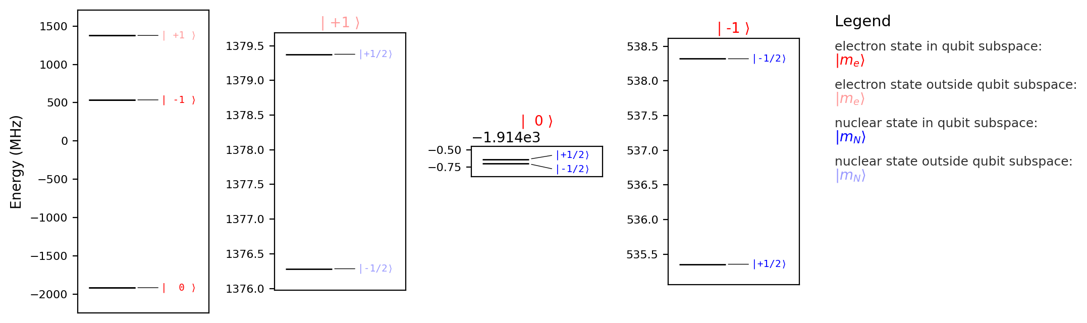
We can now visualize the energy levels of the static Hamiltonian using the plot_levels() method:

• Left subfigure: Full spectrum (\(3 \times 2\) states), dominated by the electron spin splitting.

• Three right subfigures: Splitting of the nuclear spin corresponding to the different electron spin states \(m_S = (-1, 0, 1)\).

• The plot groups the spectrum by electron-spin states and, when nuclear spins are present, shows zoom panels for the corresponding nuclear-spin structure. The current implementation supports up to three electron spins.

model.plot_levels()

Eigenenergies of the static Hamiltonian can be obtained using the eigenenergy() method. The quantum_nums must be specified as an argument. Eigenstates and eigenenergies are labeled by the quantum numbers of the product basis state that has the largest overlap with the given eigenstate. More precisely, Simphony computes the overlap matrix between eigenstates and local-\(S_z\) product-basis states, then assigns labels using a one-to-one maximal-overlap matching.

The quantum_nums should be provided as a tuple containing the quantum numbers in the same order as indicated by the spin_names attribute:

model.eigenenergy(quantum_nums=(-1,-1/2))

538.3194538083332

Alternatively, we can specify it as a dictionary, where the keys correspond to the spin names and the values correspond to the quantum numbers:

model.eigenenergy(quantum_nums={'N': -1/2, 'e': -1})

538.3194538083332

Due to the \(h = 1\) convention, energies are equivalent to frequencies and are expressed in \(\mathbf{MHz}\).

Eigenstates of the static Hamiltonian can be calculated using the eigenstate() method:

model.eigenstate(quantum_nums={'N': -1/2, 'e': -1})

array([0.+0.j, 0.+0.j, 0.+0.j, 0.+0.j, 0.+0.j, 1.+0.j])

The returned quantum state is expressed as a vector of coefficients with respect to the product basis states. The product basis states can be obtained using the productstate() method:

model.productstate(quantum_nums={'N': -1/2, 'e': -1})

array([0.+0.j, 0.+0.j, 0.+0.j, 0.+0.j, 0.+0.j, 1.+0.j])

Knowledge of the energy splittings of the model is essential for coherent control of a quantum system. We can calculate the splittings using the splitting() method:

model.splitting(spin_name='e', quantum_nums=(0,-1), rest_quantum_nums={'N': -1/2})

2453.0212188154314

The method returns the energy splitting between two eigenstates of the model. The two eigenstates must differ only in a single quantum number, which is characterized by the spin_name and its two quantum_nums. The quantum numbers of the remaining spins are provided in rest_quantum_numbers as a dictionary. There is an alternative method to calculate the splittings if we restrict ourselves to the qubit subspace, i.e., the splitting_qubit() method automatically returns the qubit splitting corresponding to the spin specified with spin_name:

splitting_m = model.splitting_qubit(spin_name='e', rest_quantum_nums={'N': -1/2})
splitting_p = model.splitting_qubit(spin_name='e', rest_quantum_nums={'N': 1/2})

[splitting_m, splitting_p]

[2453.0212188154314, 2449.9932429462215]

If rest_quantum_nums is not provided, the splitting is averaged over all possible configurations of the remaining spins, i.e., while all other spins take on every possible value from their quantum_nums set:

spitting = model.splitting_qubit(spin_name='e')
[spitting, (splitting_m + splitting_p)/2]

[np.float64(2451.5072308808267), 2451.5072308808267]

To implement quantum gates using pulses, we perform rotations on the Bloch sphere. The most common approach is to use resonant pulses with rectangular envelopes. Calculating the appropriate pulse strength or duration — given the other — is essential. The rabi_period() method determines the period of a Rabi oscillation under a constant-strength driving field, while the rabi_amplitude() method calculates the required amplitude for a given period. The rabi_period_qubit() and rabi_amplitude_qubit() variants simplify this process when working in the qubit subspace.

For example, here we calculate the strength of an AC radiofrequency driving field required to produce Rabi oscillations of the nuclear spin with a period of \(100~\mu\text{s}\):

amplitude = model.rabi_amplitude_qubit(
    driving_field_name='RF_y',
    period_time=100, # us
    spin_name='N',
    rest_quantum_nums={'e': 0}
)
print('amplitude = {} T'.format(amplitude))

amplitude = 0.00029181239941275647 T

We can check whether the amplitude corresponds to the period we set above:

period_time = model.rabi_period_qubit(
    driving_field_name='RF_y',
    amplitude=amplitude, # T
    spin_name='N',
    rest_quantum_nums={'e': 0}
)
print('period time = {} us'.format(period_time))

period time = 100.0 us

We note that times in Simphony are expressed in microseconds (\(\mu\text{s}\)).

Adding pulses

The primary purpose of Simphony is to simulate the time evolution of a spin register governed by time-dependent pulse sequences. Users can add pulses to driving fields. Driving fields can be accessed from the model via the driving_fields attribute (which provides a list of driving field objects) or using the driving_field(name: str) method, which returns the corresponding field. The names of all driving fields are stored in the driving_field_names attribute.

In this tutorial, we use rectangular pulses exclusively. Due to the hyperfine interaction, the electron spin energy splitting depends on the nuclear spin state, making it nontrivial to apply a pulse that is resonant with the electron spin regardless of the state of the nuclear spin. To address this, the pulse frequency is set to the average electron splitting for the two nuclear spin states. A strong driving field (with Rabi frequency greater than the hyperfine interaction strength) ensures that the electron spin can be rotated irrespective of the nuclear spin state. The pulse duration is chosen as half of the Rabi period, thereby realizing a \(\pi\) rotation:

amplitude = 0.004 # T
splitting_frequency_e = model.splitting_qubit('e')
phase = 0
duration = 0.5 * model.rabi_period_qubit('MW_x', amplitude, 'e')

model.driving_field('MW_x').add_rectangle_pulse(
    amplitude=amplitude,
    frequency=splitting_frequency_e,
    phase=phase,
    duration=duration
)

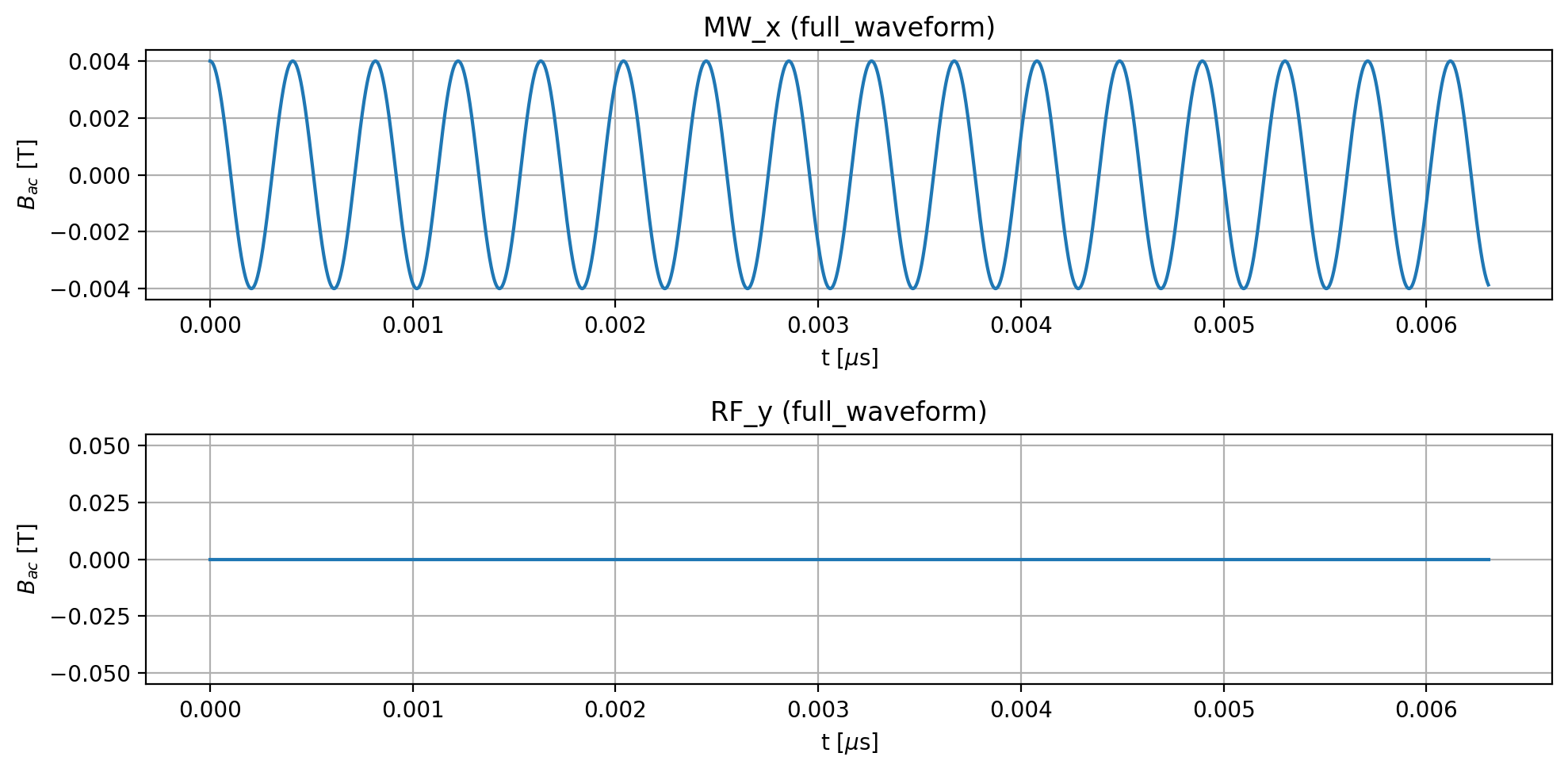
To visualize the driving fields, use the plot_driving_fields() method:

model.plot_driving_fields()

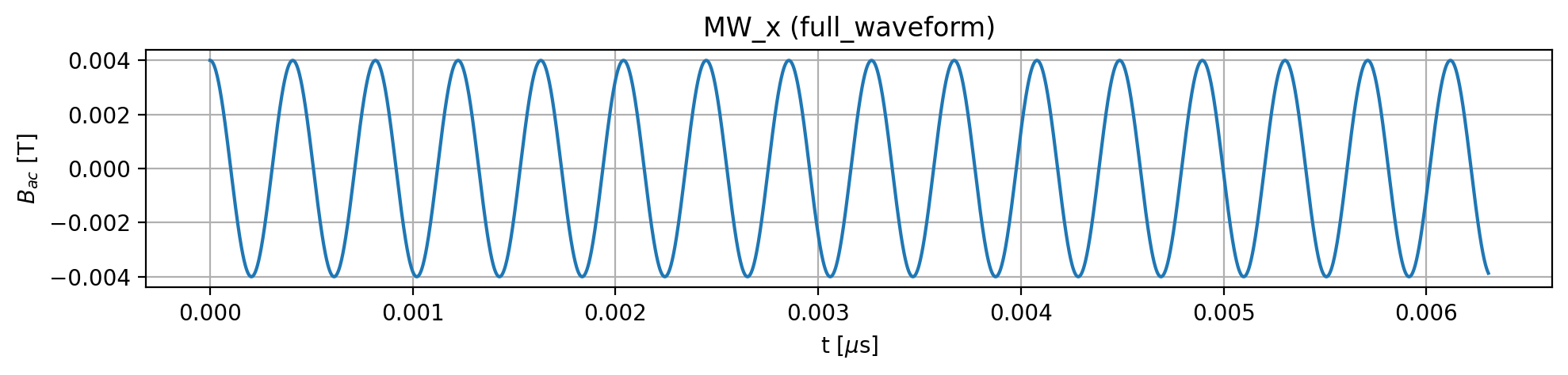
To plot a specific driving field, select it by name and use the plot_pulses() method:

model.driving_field('MW_x').plot_pulses()

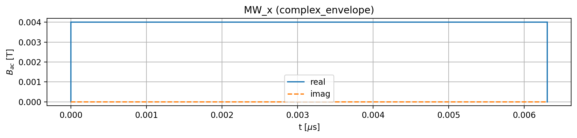
To display only the complex envelope of the pulse, use the function='complex_envelope' option (by default: function='full_waveform'):

model.driving_field('MW_x').plot_pulses(function='complex_envelope')

You can reset all driving fields using the remove_all_pulses() method (not executed here):

# model.remove_all_pulses()

The remove_all_pulses() method removes all pulses from the driving fields, but the driving fields themselves remain in the model.

An alternative way to add pulses to the model is by using the Pulse class:

pulse1 = simphony.Pulse(
    start=1,
    end=2,
    frequency=splitting_frequency_e,
    complex_envelope=0.01 + 0.02 * 1j
)

The complex_envelope can be provided as a Python function (callable):

def complex_envelope_fn(t):
    return 0.01 * 1j * np.exp(t)

pulse2 = simphony.Pulse(
    start=2.5,
    end=3,
    frequency=splitting_frequency_e,
    complex_envelope=complex_envelope_fn
)

And you can simply add the pulse using the add_pulse() method (not executed here):

# model.driving_field('MW_x').add_pulse(pulse2)

Rotating frame

The rotating frame is often introduced to simplify the description of the time evolution of quantum systems. Gates realized by pulse sequences are usually interpreted in the rotating frame. In Simphony, the operator corresponding to the rotating frame has the form:

\[ U_\text{rotating}(t) = \bigotimes_{i \in \text{spins}} e^{i 2\pi f_i t \sigma_{z,i} / 2}. \]

By default, a Model can manage these frequencies automatically through a RotatingFrameSetter. That automatic mode is the recommended default in higher-level workflows, because the rotating-frame choice stays attached to the model configuration and is updated consistently when the model is rebuilt. For more details, see the API documentation.

In this low-level example we switch to manual control and then set the electron rotating-frame frequency to the excitation frequency:

model.rotating_frame = None
spin_e.rotating_frame_frequency = splitting_frequency_e

The rotating-frame frequencies can then be retrieved together using:

model.rotating_frame_frequencies

array([2451.5072,    0.    ])

Simulations are still propagated in the lab frame. The rotating frame only changes how operators and states are reported and interpreted during analysis.

Running Simulations

The primary functionality of Simphony is running simulations. This is currently done by solving the time-dependent Schrödinger equation in an exact way (without the rotating wave approximation). As a result, the time-dependent evolution operator is computed exactly and made available for further analysis.

Simphony is designed to simulate pulse sequences composed of microwave and radio-frequency pulses, usually applied alternately. In the background, the simulated pulse sequence is divided into time segments defined by the start and end boundaries of each pulse. Each time segment is associated with the pulses active during that segment. The time-dependent Schrödinger equation is solved over these segments using a discretized approach. The resolution is set according to the highest pulse frequency, with time steps corresponding to one 250th (by default) of its period. If a time segment contains a single pulse with a constant envelope, Simphony simplifies the simulation: only a single period of that sine wave is simulated and used to reconstruct the full pulse time evolution.

The simulate_time_evolution() method, when called without parameters, runs a default simulation. However, it is highly customizable. The most important parameters include:

• end: The end time of the simulation (default: end of the last pulse)

• n_eval: The number of time points returned per simulation segment (default: 251)

• simulation_method: It must be 'basic' or 'single_sine_wave' (default: 'single_sine_wave')

• n_split: Number of split points per time segments (default: 250)

• apply_noise: Whether to include noise in the simulation (default: True)

• n_shots: For noisy simulations, the number of different noise realizations (default: 1)

The simulate_time_evolution() method returns the simulation results as an instance of the SimulationResult class:

result = model.simulate_time_evolution(verbose=True)
result

start = 0.0
end = 0.006306005885393217
solver_method = numpy_expm
number of simulated driving terms = 1
number of simulated noise terms = 0
---------------------------------------------------------------------------
simulate time segment [0.00000, 0.00631] with step size 1.632e-06 (type: single_sine_wave)

SimulationResult(model_dimension=6, n_shots=1, n_ts=251)

It is important to note that the simulation time strongly depends on the number of returned time points, which is controlled by the n_eval parameter. If only the final result of the pulse sequence is needed, setting n_eval=2 can significantly speed up the simulation. However, even in this case, Simphony may still return intermediate results at the end of each simulation segment, not only at the final time point.

The returned instance stores the main details of the simulation:

• model: the simulated model

• ts: timestamps of the stored simulation data

• time_evol_operator: time-evolution operator corresponding to the dynamics (by default, this is the direct result of the simulation)

The time-evolution operators are stored as an instance of the TimeEvolOperator class:

result.time_evol_operator

TimeEvolOperator(dimension=6, n_shots=1, n_ts=251)

The matrix representation of the time-evolution operator can be obtained using the matrix() method. Its arguments are:

• basis: must be either 'product' or 'eigen'

• frame: must be either 'lab' or 'rotating'

• t_idx: indices of the time points

• shot: index or indices of the shots (see later)

result.time_evol_operator.matrix(basis='eigen', frame='rotating', t_idx=[0,-1], shot=[0])

array([[[[ 1.0000e+00+0.0000e+00j,  0.0000e+00+0.0000e+00j,  0.0000e+00+0.0000e+00j,  0.0000e+00+0.0000e+00j,  0.0000e+00+0.0000e+00j,  0.0000e+00+0.0000e+00j],
         [ 0.0000e+00+0.0000e+00j,  1.0000e+00+0.0000e+00j,  0.0000e+00+0.0000e+00j,  0.0000e+00+0.0000e+00j,  0.0000e+00+0.0000e+00j,  0.0000e+00+0.0000e+00j],
         [ 0.0000e+00+0.0000e+00j,  0.0000e+00+0.0000e+00j,  1.0000e+00+0.0000e+00j,  0.0000e+00+0.0000e+00j,  0.0000e+00+0.0000e+00j,  0.0000e+00+0.0000e+00j],
         [ 0.0000e+00+0.0000e+00j,  0.0000e+00+0.0000e+00j,  0.0000e+00+0.0000e+00j,  1.0000e+00+0.0000e+00j,  2.1684e-19+0.0000e+00j,  0.0000e+00+0.0000e+00j],
         [ 0.0000e+00+0.0000e+00j,  0.0000e+00+0.0000e+00j,  0.0000e+00+0.0000e+00j,  2.1684e-19+0.0000e+00j,  1.0000e+00+0.0000e+00j,  0.0000e+00+0.0000e+00j],
         [ 0.0000e+00+0.0000e+00j,  0.0000e+00+0.0000e+00j,  0.0000e+00+0.0000e+00j,  0.0000e+00+0.0000e+00j,  0.0000e+00+0.0000e+00j,  1.0000e+00+0.0000e+00j]],

        [[-2.3714e-01+9.6873e-01j,  7.6602e-06+1.6397e-06j, -1.1206e-02+5.0821e-02j,  2.0164e-07+1.2433e-06j,  3.4836e-02-3.7584e-02j, -1.1409e-06+4.6508e-07j],
         [ 5.6304e-06+1.9618e-06j, -3.5342e-01+9.3250e-01j,  2.7550e-05-1.4812e-06j, -1.8968e-02+5.0453e-02j,  6.2566e-06-2.0634e-05j,  3.2396e-02-3.9758e-02j],
         [ 5.0790e-02+7.7175e-03j,  1.5976e-05+1.4900e-05j, -1.7738e-03+4.8294e-03j,  1.0124e-06+2.6966e-07j,  7.8692e-01+6.1489e-01j, -7.9922e-06+1.1691e-05j],
         [-1.1467e-06+8.1623e-07j,  5.0968e-02+1.5396e-02j, -5.0712e-07-6.4702e-07j, -3.1764e-02-1.8032e-02j, -9.8262e-06+1.0876e-05j,  8.2010e-01+5.6856e-01j],
         [-4.0315e-02-3.2711e-02j,  2.3698e-05-1.2215e-05j,  7.8672e-01+6.1509e-01j,  6.7206e-06-8.4985e-06j, -3.2755e-03+5.3710e-03j, -4.2209e-07+1.2917e-07j],
         [-1.2686e-06-3.3554e-07j, -4.2379e-02-3.0078e-02j,  5.7932e-06-7.5665e-06j,  8.2009e-01+5.6852e-01j,  1.1006e-07+1.7292e-07j,  2.9685e-02+2.5642e-02j]]]])

The returned np.array has 4 dimensions: axis 0 corresponds to different shots, axis 1 to time points, and axes 2 and 3 represent the time-evolution operator as a matrix.

Using the result object, you can calculate and visualize:

• the expectation values of operators during the time evolution starting from an initial state

• the process matrix corresponding to the final propagator

• the average gate fidelity with respect to an ideal gate

Note: The result object stores a copy of the model object, rather than the original.

Expectation values

Before calculating expectation values, an initial state must be defined. Note that this can be done even after the simulation has finished: simulate_time_evolution() computes the time-evolution operator, and once that operator is available, the corresponding state trajectory for a chosen initial state can be obtained without rerunning the simulation:

result.initial_state = model.productstate({'e': 0, 'N': -1/2})

In the background, the time-evolved states corresponding to the time points are computed using the time-evolution operators:

result.time_evol_state

TimeEvolState(dimension=6, n_shots=1, n_ts=251)

To calculate expectation values, use the expectation_value() method. The operator should be provided as an np.array whose dimensions match the model’s full Hilbert space. Alternatively, if you only want to apply the operator within the qubit subspace, set in_qubit_subspace=True. In that case, the operator should match the size of the qubit subspace.

Another option is to specify the operator as a Pauli string acting on the qubit subspace of the spin register. The order of qubits should correspond to model.spin_names. Note that any operator input can also be provided as a list of such operators.

For example, we can calculate the Bloch vector components of the electron spin at the first and last timestamps as follows:

result.expectation_value(['XI','YI','ZI'], t_idx=[0,-1])

array([[[ 0.    ,  0.    ,  1.    ],
        [-0.0726, -0.0065, -0.9944]]])

The shape corresponds to shots × time points × operators. By default, the calculation is performed in the product basis and in the rotating frame. Without retrieving the numerical values, we can plot the expectation values at once (here in the lab frame):

result.plot_expectation_value(['XI','YI','ZI'], frame='lab')

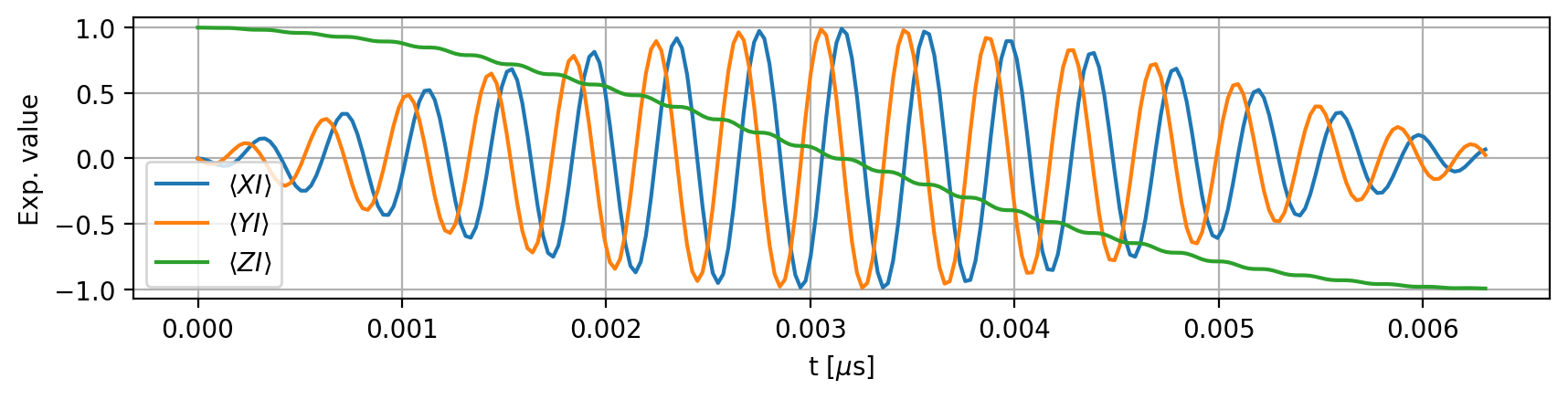
Bloch vectors are derived from the expectation values of the Pauli matrices. We can plot the Bloch vectors for all spins as follows:

result.plot_Bloch_vectors()

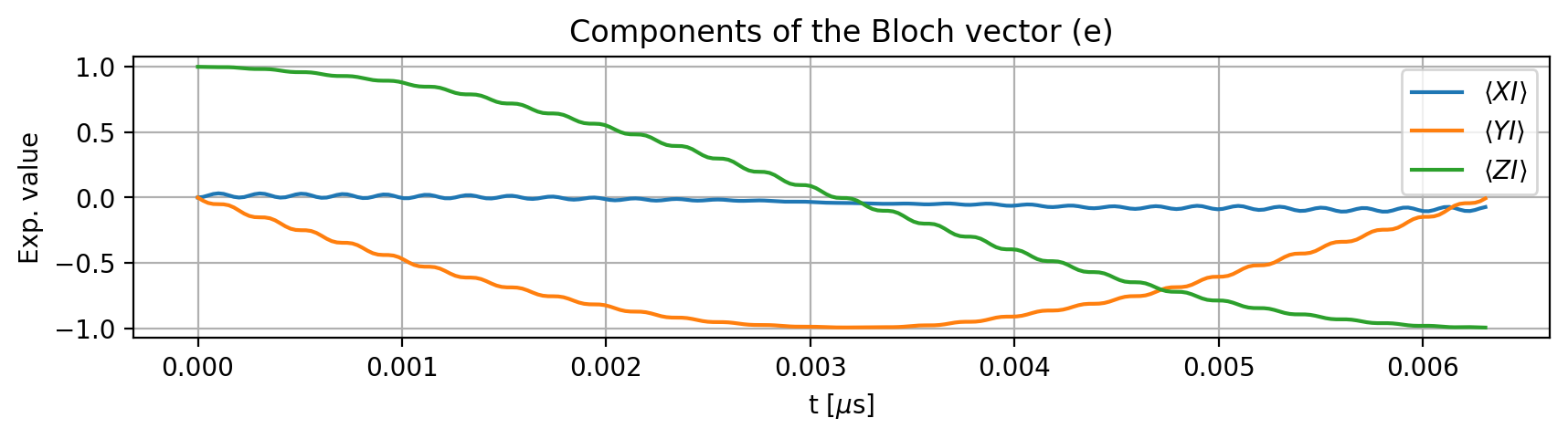
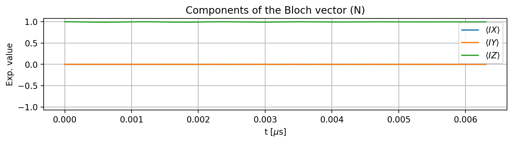
By default, the method uses the rotating frame and the product basis to plot the Bloch vectors.

Process matrix

The process matrix is one of the most informative ways to characterize and visualize quantum processes (in our case, to characterize the time evolution in the qubit subspace). Usually, it is defined via a quantum channel acting on a density matrix as:

\[ \varepsilon(\rho) = \frac{1}{2^n}\sum_{i,j=0}^{4^n-1}{\chi_{i,j} P_i \rho P_j}, \]

where \(P\)-s are the \(n\)-qubit Pauli basis elements (Pauli strings), and \(\chi_{i,j}\) is the complex-valued \(\chi\)-matrix on the Pauli basis (process matrix), whose real and imaginary parts both fall within the range \([-1, 1]\).

The process_matrix() method calculates the process matrix in a given basis and frame. With the t_idx argument, you can control the time point at which the process matrix is calculated. By default, it is set to -1, the endpoint of the time evolution. The spin_names argument can be used to restrict the spins included in the analysis:

result.process_matrix(basis='product', frame='rotating', spin_names='e')

array([[ 2.5013e-05+0.0000e+00j,  1.2304e-03+4.6388e-03j,  1.5265e-07+3.6240e-07j, -2.7234e-05-6.8412e-05j],
       [ 1.2304e-03-4.6388e-03j,  9.9655e-01+0.0000e+00j,  6.6963e-05-1.7464e-05j, -1.8594e-02+5.5751e-04j],
       [ 1.5265e-07-3.6240e-07j,  6.6963e-05+1.7464e-05j,  1.2134e-08+0.0000e+00j,  1.9517e-07-2.8194e-07j],
       [-2.7234e-05+6.8412e-05j, -1.8594e-02-5.5751e-04j,  1.9517e-07+2.8194e-07j,  7.1077e-04+0.0000e+00j]])

You can plot the process matrix directly using the plot_process_matrix() method. There are two options:

• value='re-im' to plot the real and imaginary parts of the complex process matrix

• value='abs' to plot its absolute value

result.plot_process_matrix(value='re-im', basis='product', frame='rotating')

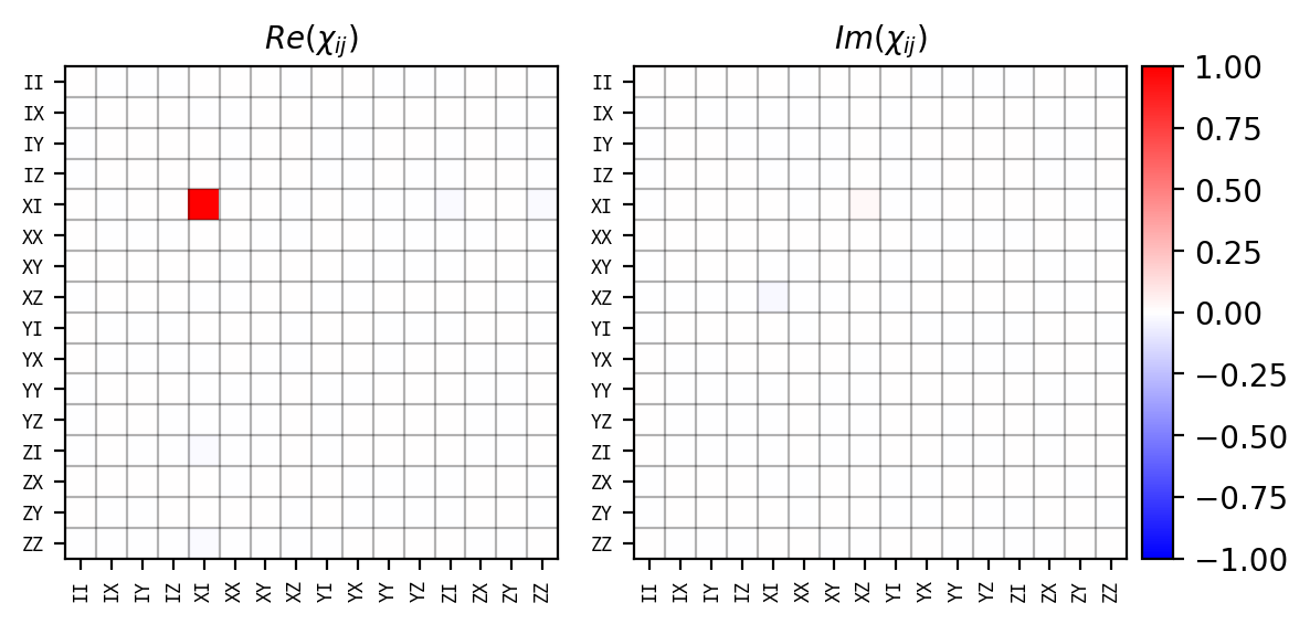
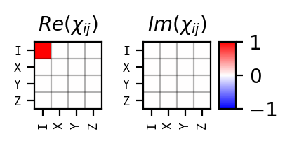
One also can control the visualized time point by the t_idx argument. For example, t_idx=0 yields to an identity operation:

result.plot_process_matrix(value='re-im', t_idx=0, basis='product', frame='rotating', spin_names='e')

Average gate fidelity

The average gate fidelity measures how closely the implemented gate or circuit matches the ideal one. Before calculating it, you need to define the ideal quantum gate or circuit to serve as a reference. This will be compared against the gate or circuit realized via time evolution. To do this, import Qiskit’s QuantumCircuit class and define the quantum circuit using gates:

from qiskit import QuantumCircuit

qc = QuantumCircuit(2)
qc.x(0)
qc.draw()

     ┌───┐
q_0: ┤ X ├
     └───┘
q_1: ─────
          

To calculate the average gate fidelity, add the qc to the result object:

result.ideal = qc

This automatically computes the ideal unitary operator:

result.ideal_unitary_matrix

array([[0.+0.j, 0.+0.j, 1.+0.j, 0.+0.j],
       [0.+0.j, 0.+0.j, 0.+0.j, 1.+0.j],
       [1.+0.j, 0.+0.j, 0.+0.j, 0.+0.j],
       [0.+0.j, 1.+0.j, 0.+0.j, 0.+0.j]])

The average gate fidelity can be calculated using:

result.average_gate_fidelity()

np.float64(0.9965842246023643)

When the average gate fidelity is calculated, the averaging is performed over the pure states of the qubit subspace.

The resulting average gate fidelity is very close to \(1\), indicating that the pulse effectively implements an unconditional single-qubit \(\text{RX}(\pi)\) gate within the electron spin qubit subspace. The small deviation from perfect fidelity arises from a weak — though not infinitesimally weak — driving field, which leads to non-ideal Rabi oscillations (as described by the Bloch–Siegert shift). Simphony simulates the exact time evolution, allowing such subtle errors to be revealed and analyzed.

Where to go next

Congratulations on completing the basic tutorial! Here are the recommended follow-up notebooks to deepen your knowledge of Simphony:

Introductory tutorials

• 2_tutorial_default_nv_models.ipynb: Explore the high-level NV model builders and hyperfine database. Learn how to configure realistic multi-spin systems with carbon isotopes.

• 3_tutorial_autodiff_gate_optimization.ipynb: Introduction to automatic differentiation (autodiff) and pulse optimization using JAX. Optimize simple pulse sequences with gradient descent.

• 4_tutorial_single_sine_wave_method.ipynb: Efficient pulse generation method for constant-envelope driving fields. A key technique for realistic experiments.

Advanced examples

• 5_example_knight_field.ipynb: Modeling Knight-shift field effects and their role in multi-spin dynamics.

• 6_example_ramsey_with_quasistatic_noise.ipynb: Noise-aware simulation. Learn how to model local quasistatic noise and analyze its effects on coherence.

• 7_example_multiqubit_phase_gate_autodiff.ipynb: Advanced multiqubit gate optimization. Combine autodiff with realistic gate fidelity analysis.

• 8_example_pulsed_odmr.ipynb: Optically detected magnetic resonance (ODMR) simulation. Realistic signal acquisition and detection.

• 9_example_dc_magnetometry.ipynb: DC magnetometry for external field sensing. Robust pulse optimization for magnetometer sequences.

• 10_example_ac_magnetometry.ipynb: AC magnetometry techniques for enhanced field sensitivity.