Knight field - Effective Nuclear Gyromagnetic Ratio (\(^{14}\)N in NV Center)

Description of the effect

When one aims to drive the nuclear spin - for simplicity, in our case the \(^{14}N\) nuclear spin - an interesting effect occurs: The direct driving through the \(\gamma_n\mathbf{B}(t)\mathbf{I}\) interaction term is weaker than an indirect driving. The indirect driving is through the strongly off-resonant driving of the electronic spin, and the spin - spin interaction term \(\mathbf{S\,A\,I}\). The driving - which is resonant for the nitrogen, and very slow for the electronic spin - causes the electronic spin to oscillate, and the induced magnetic field of the electronic spin interacts with the nuclear spin through the hyperfine interaction.
Crucial ingredients of such a phenomenon are the nonzero transverse \(A_{xx},\, A_{yy}\) components of the hyperfine tensor (with the \(z-\)axis is conveniently chosen to be parallel with the NV axis), which supply the \(S_x I_x\) / \(S_y I_y\) coupling that converts the electron’s oscillation into a transverse field on the nucleus.

Description 1: An intuitive understanding

Consider the following Hamiltonian:

(1)\[\begin{equation} H = D S_z^2 + \gamma_e \mathbf{B}_0\mathbf{S}+ P I_z^2 - \gamma_n \mathbf{B}_0\mathbf{I}+\mathbf{SAI} + \gamma_e \mathbf{B}_{\text{drive}}(t)\mathbf{S}+ \gamma_n \mathbf{B}_{\text{drive}}(t)\mathbf{I}. \end{equation}\]

Here both spins are spin-1, and the physical constants are the following:

• \(D = 2.872 \,\text{GHz}\) zero-field splitting,

• \(\gamma_e = 28.0331 \,\text{GHz/T}\) electron gyromagnetic ratio,

• \(P = -5.01 \,\text{MHz}\) nitrogen quadrupole moment,

• \(\gamma_n = 3.07771 \,\text{MHz/T}\) nitrogen gyromagnetic ratio (for N-14),

• \(\mathbf{A} = \begin{pmatrix} A_{xx} && \\ & A_{yy} &\\ && A_{zz} \end{pmatrix}\) hyperfine tensor with \(A_{xx} = A_{yy} = -2.7 \,\text{MHz}\) hyperfine perpendicular and \(A_{zz} = -2.14 \,\text{MHz}\) hyperfine parallel terms.

If the electronic spin is locked in a certain manifold (e.g. \(m_S = 0\) or \(m_S = -1\)), by optical pumping and/or MW control and electronic spin transitions are far off‑resonant from the RF, one can replace \(\mathbf{S}\) by its expectation value \(\langle\mathbf{S}\rangle\) in that manifold and obtain an effective nuclear Hamiltonian:

(2)\[\begin{equation} H_{\text{nucl, eff}} = -\gamma_n \mathbf{B}_0\mathbf{I}+\langle\mathbf{S}\rangle\mathbf{AI} + \gamma_n \mathbf{B}_{\text{drive}}(t)\mathbf{I}. \end{equation}\]

The Knight field is the effective field that acts on the nuclear spin, through the off-resonant oscillation:

(3)\[\begin{equation} \mathbf{B}_K = -\gamma_n^{-1} \langle \mathbf{S}\rangle \mathbf{A}. \end{equation}\]

To compute the effective description of the electronic spin expectation value, consider the following effective electronic spin Hamiltonian (neglecting the Overhauser field - nuclear spin’s effect on the electron through the hyperfine interaction):

(4)\[\begin{align} H_{e,\text{eff}} &= DS_z^2 + \gamma_e \mathbf{B}_0\mathbf{S} + \gamma_e \mathbf{B}_{\text{drive}}(t)\mathbf{S}, \\ \mathbf{B}_{\text{drive}}(t) &= B_{d} \cos(\omega_dt) \hat{\mathbf{x}}. \end{align}\]

Assume \(\mathbf{B}_0 \parallel \mathbf{z}\). The effective electronic Hamiltonian in matrix form:

(5)\[\begin{align} H_{e,\text{eff}} = \begin{pmatrix} D +\gamma_e B_0 & & \\ & 0 & \\ & & D -\gamma_e B_0 \end{pmatrix} + \gamma_e B_d \cos(\omega_d t) \frac{1}{\sqrt{2}} \begin{pmatrix} & 1 & \\ 1& & 1\\ & 1 & \end{pmatrix}. \end{align}\]

There are a few ways to derive the oscillation of the spin, e.g.:

• Consider a 2 dimensional restricted subspace of the Hilbert space, and use standard off-resonant Rabi oscillation results.

• Treat the time-dependent term as an adiabatic perturbation, and use standard perturbation theory.

Rabi oscillation description

Since the \(|+1\rangle \leftrightarrow |-1\rangle\) transition is forbidden in first order, and given that the driving amplitude is weak (\(\gamma_e B_d \ll D \pm \gamma_e B_0\)), the system can be effectively restricted to isolated two-level subspaces: either \(\{|+1\rangle, |0\rangle\}\) or \(\{|-1\rangle, |0\rangle\}\), depending on the driving frequency. In the restricted subspaces, the problem is a standard driven spin-1/2, i.e. the off-resonant Rabi oscillation. Applying this approach:

• Use results from the off-resonant Rabi oscillation: For the effective spin \(-\frac{1}{2}\) model with

  (6)\[\begin{align} H_{e,\text{eff},1/2} &= \begin{pmatrix} \Delta/2 & \\ & -\Delta/2 \end{pmatrix} + \gamma_e B_d \cos(\omega_d t) \frac{1}{\sqrt2} \begin{pmatrix} & 1 \\ 1 & \end{pmatrix} \\ \Delta &= D \pm \gamma_e B_0 \qquad \text{for } m_S = \pm 1 \end{align}\]

  In this case the off-resonant oscillation between the two states is:

  (7)\[\begin{equation} P_{1\rightarrow 2}(t) = \frac{4|\gamma_e B_d \frac{1}{\sqrt{2}}|^2}{\Delta^2 + 4|\gamma_e B_d \frac{1}{\sqrt{2}}|^2} \sin^2 \left( \frac12 t \sqrt{\Delta^2 + 4|\gamma_e B_d \frac{1}{\sqrt{2}}|^2}\right) \end{equation}\]

First Order Perturbation Theory

As the driving is much slower than the electronic spin’s resonant driving, we can assume the electronic spin’s time evolution follows the instantaneous eigenstates. The exact instantaneous eigenstates are fairly difficult to compute, hence we can approximate with (time-independent) first order perturbation theory:

(8)\[\begin{align} | 1 \rangle^{(1)} &= \begin{pmatrix} 1 \\ 0 \\ 0 \end{pmatrix} + \frac{1}{\sqrt{2}}\frac{\gamma_e B_d\cos(\omega_dt)}{D+\gamma_e B_0} \begin{pmatrix} 0 \\ 1 \\ 0 \end{pmatrix}, \\ | 0 \rangle^{(1)} &= \begin{pmatrix} 0 \\ 1 \\ 0 \end{pmatrix} + \frac{\gamma_e B_d\cos(\omega_dt)}{\sqrt{2}}\left[\frac{1}{-(D+\gamma_e B_0)} \begin{pmatrix} 1 \\ 0 \\ 0 \end{pmatrix} + \frac{1}{-(D-\gamma_e B_0)} \begin{pmatrix} 0 \\ 0 \\ 1 \end{pmatrix} \right], \\ | -1 \rangle^{(1)} &= \begin{pmatrix} 0 \\ 0 \\ 1 \end{pmatrix} + \frac{1}{\sqrt{2}}\frac{\gamma_e B_d\cos(\omega_dt)}{D-\gamma_e B_0} \begin{pmatrix} 0 \\ 1 \\ 0 \end{pmatrix}. \end{align}\]

Through straightforward algebra, we compute the magnetization expectation values for the three perturbed eigenvalues, in 1st order:

(9)\[\begin{align} \langle 1|^{(1)}\mathbf{S}|1\rangle^{(1)}(t) &= \left(\frac{\gamma_e B_d\cos(\omega_d t)}{D+\gamma_eB_0}{}\,, 0,\, 1\right)^T,\\ \langle 0|^{(1)}\mathbf{S}|0\rangle^{(1)}(t) &= \left( -\frac{2D\gamma_e B_d\cos(\omega_d t)}{D^2-(\gamma_eB_0)^2},\, 0,\, 0 \right)^T,\\ \langle -1|^{(1)}\mathbf{S}|-1\rangle^{(1)}(t) &= \left( \frac{\gamma_e B_d\cos(\omega_d t)}{D-\gamma_eB_0}{}\,, 0,\, -1\right)^T. \end{align}\]

The \(\mathbf{B}_K = -\gamma_n^{-1}\langle \mathbf{S}\rangle \mathbf{A} \) Knight field follows:

(10)\[\begin{align} \mathbf{B}_K &= \frac{\gamma_e}{\gamma_n} \frac{A_{xx}} {D+\gamma_eB_0}B_d\cos(\omega_d t)\hat{\mathbf{x}}, \qquad \text{for $m_S = 1$},\\ \mathbf{B}_K &= -\frac{\gamma_e}{\gamma_n} \frac{2A_{xx}D}{D^2-(\gamma_eB_0)^2} B_d\cos(\omega_d t)\hat{\mathbf{x}}, \qquad \text{for $m_S = 0$},\\ \mathbf{B}_K &= \frac{\gamma_e}{\gamma_n}\frac{A_{xx} }{D-\gamma_eB_0}B_d\cos(\omega_d t)\hat{\mathbf{x}}, \qquad \text{for $m_S = -1$}. \end{align}\]

Note: In the Rabi oscillation based description, one recovers the same results for \(m_S = \pm 1\) if the solution is expanded in first order.

Description 2: A more direct derivation

While quantitatively the same, a different way of thinking is the following: Assuming other transitions are very off-resonant, a transition between two states is always driven by the respective off-diagonal matrix element of the Hamiltonian. Hence, in the spirit of Rabi oscillation, we compute the matrix elements of the Hamiltonian between the \(I_z = 0, \, \pm 1\) nuclear states. Due to the hyperfine interaction, and more precisely the \(A_{xx},\, A_{yy}\) perpendicular terms, \(I_z\) does not commute with the Hamiltonian, hence the \(I_z\) eigenstates are not eigenstates of \(H\). We consider this in first order perturbation theory, and compute the matrix elements of the Hamiltonian between the perturbed eigenstates.

Numerical tests involving Simphony

import matplotlib.pyplot as plt
import numpy as np
import simphony

simphony.Config.set_matplotlib_format('retina')
np.set_printoptions(linewidth=200, precision=4)

b0 = 0.05 # in Tesla, we define as a variable as it will be used also in the analytical expressions for the Knight field.
model = simphony.default_nv_model(nitrogen_isotope=14,
                                  static_field_strength=b0)
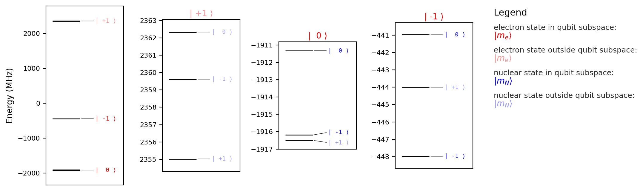
model.plot_levels()

Rabi oscillations

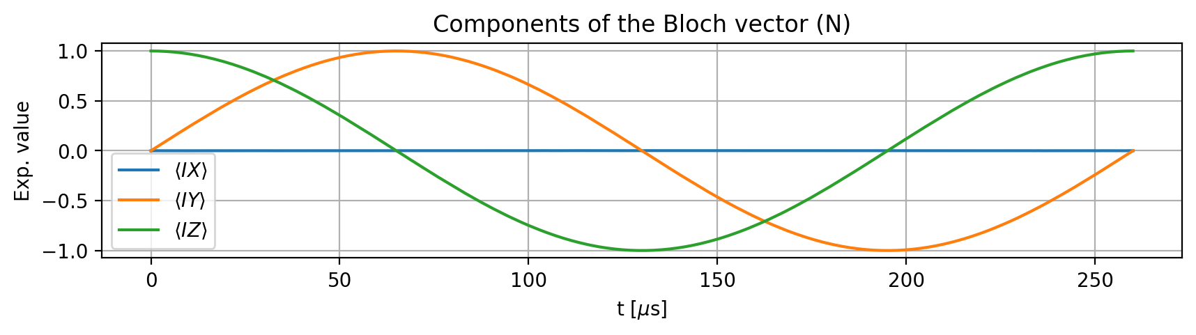
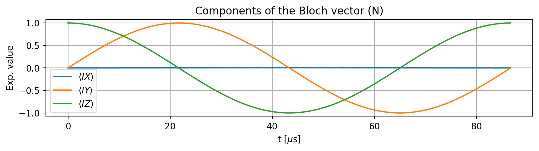
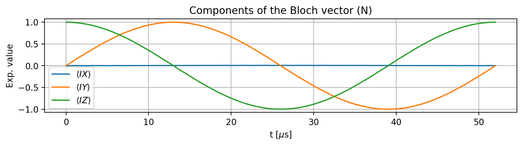
Simphony inherently takes care of the indirect driving through hyperfine interaction. This is highlighted by the application of the .rabi_cycle_amplitude(), .rabi_cycle_amplitude_qubit(), rabi_cycle_time(), .rabi_cycle_time_qubit() methods: They compute the amplitude or period required for resonant driving to achieve a \(2\pi\) rotation in the specified transition. They compute this by considering the matrix element between the involved eigenstates (labelled by spin quantum numbers).

These methods give consistent results across a wide range of amplitudes and periods. Deviations are due to leakage and Bloch-Siegert oscillations.

# demonstrate the goodness of built-in methods

initial_nitrogen_idx = 0        # labeled by the I_z quantum number, for 14N, the possible values are -1, 0, and +1. Qubit subspace is {0, -1}. 
transition_nitrogen_idx = -1    # as above
electron_idx = -1               # labeled by the S_z quantum number, the possible values are -1, 0, and +1. Qubit subspace is {0, -1}: {|0>, |1>}, respectively. 
for amplitude in [0.0001, 0.0003, 0.0005, 0.001, 0.002, 0.005, 0.01, 0.02, 0.05]:
    model.remove_all_pulses()
    frequency = model.splitting(spin_name='N',
                                quantum_nums=[initial_nitrogen_idx, transition_nitrogen_idx],
                                rest_quantum_nums={'e': electron_idx})
    duration = model.rabi_period(driving_field_name='RF_x',
                                 amplitude=amplitude,
                                 spin_name='N',
                                 quantum_nums=[initial_nitrogen_idx, transition_nitrogen_idx],
                                 rest_quantum_nums={'e': electron_idx})
    model.driving_field('RF_x').add_rectangle_pulse(amplitude=amplitude,
                                                    frequency=frequency,
                                                    phase=0.0,
                                                    duration=duration)
    coherent_result = model.simulate_time_evolution(apply_noise=False)
    coherent_result.initial_state = model.productstate({'e': electron_idx, 'N': initial_nitrogen_idx})
    print(f"Amplitude: {amplitude}")
    coherent_result.plot_Bloch_vectors(frame='rotating', spin_names=['N'])
    plt.show()

Amplitude: 0.0001

Amplitude: 0.0003

Amplitude: 0.0005

Amplitude: 0.001

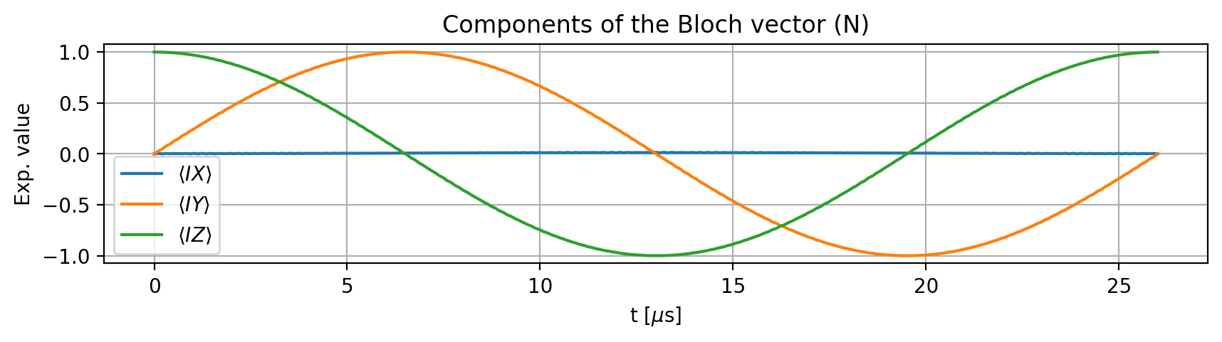
Amplitude: 0.002

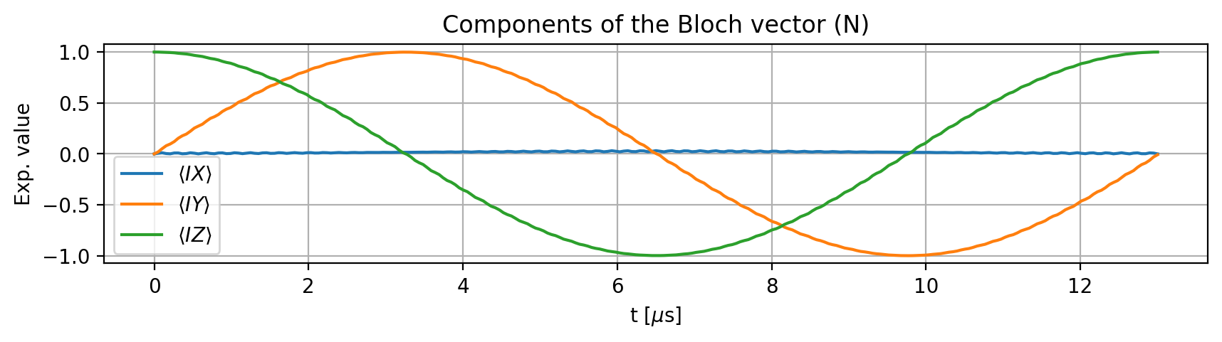
Amplitude: 0.005

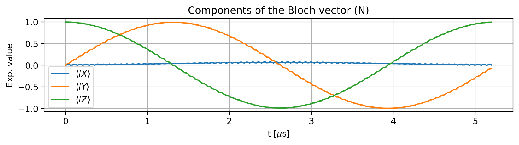
Amplitude: 0.01

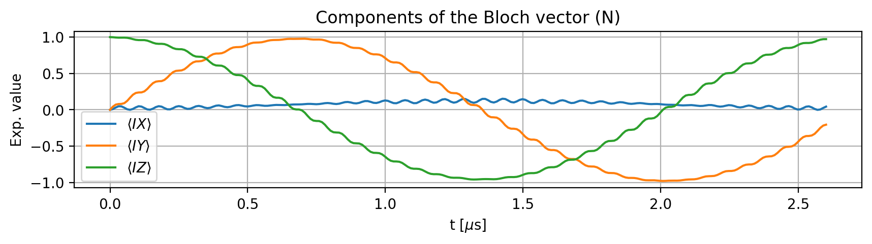
Amplitude: 0.02

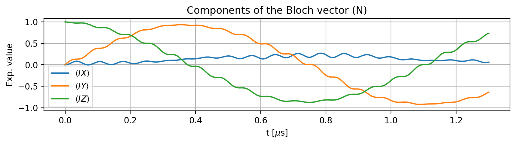
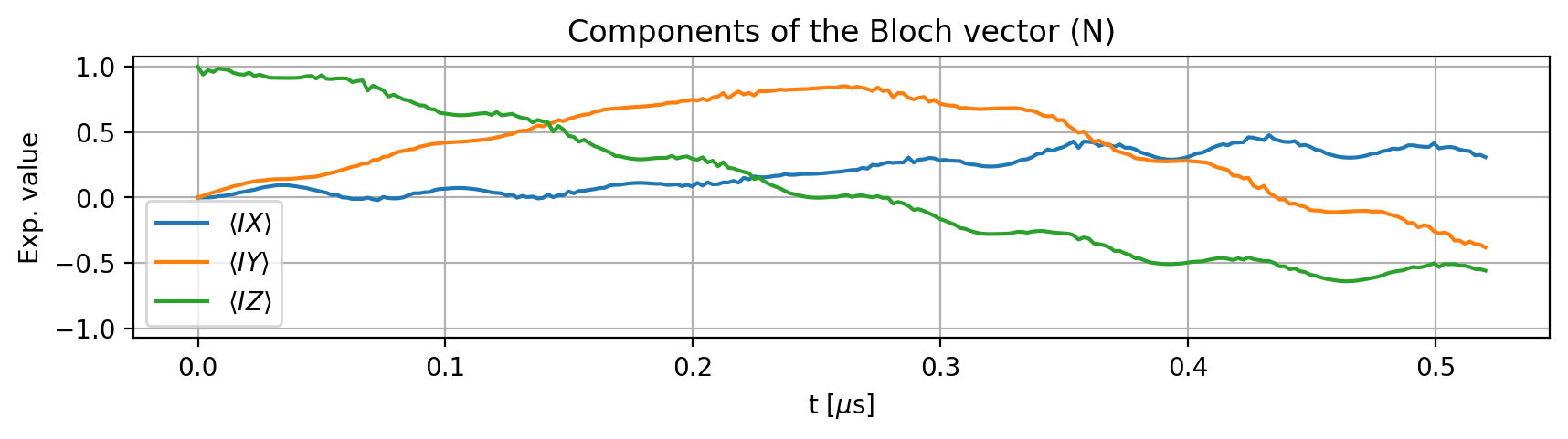
Amplitude: 0.05

Comparison of effective nuclear gyromagnetic ratios (analytical and numerically exact)

To directly compare the perturbative analytical result to the numerically exact Simphony result, the most instructive is to express the effective gyromagnetic ratio of the nucleus, which drives the nitrogen nuclear spin through the \(H_{RF} = \gamma_{n,\text{eff}} \mathbf{B}_d(t)\mathbf{I}\):

(11)\[\begin{align} \gamma_{n,\text{eff}} &= -\gamma_n + \frac{\gamma_e A_{xx}} {D+\gamma_eB_0} \qquad \text{for $m_S = 1$}\\ \gamma_{n,\text{eff}} &= -\gamma_n - \frac{2\gamma_e A_{xx}D}{D^2-(\gamma_eB_0)^2} \qquad \text{for $m_S = 0$}\\ \gamma_{n,\text{eff}} &= -\gamma_n + \frac{\gamma_e A_{xx} }{D-\gamma_eB_0} \qquad \text{for $m_S = -1$} \end{align}\]

On the Simphony side, it is easiest to extract model.matrix_element(), which computes the matrix element of the time-independent (pulse-independent) part of the driving operator. Note the \(\sqrt{2}\) difference, which comes from the spin-1 \(I_x\) matrix.

initial_nitrogen_idx = 0        # labeled by the I_z quantum number, for 14N, the possible values are -1, 0, and +1. Qubit subspace is {0, -1}. 
transition_nitrogen_idx = -1    # as above

# define the physical constants for the analytical expressions from the model
gamma_n = model.spin('N').gyromagnetic_ratio
gamma_e = model.spin('e').gyromagnetic_ratio
d = model.spin('e').zero_field_splitting
a_perpendicular = model.interactions[0].xx

numerical_eff_gyrom_ratio_e_p1 = model.matrix_element(driving_field_name='RF_x',
                                                      state1=model.eigenstate(quantum_nums={'e': 1, 'N': initial_nitrogen_idx}),
                                                      state2=model.eigenstate(quantum_nums={'e': 1, 'N': transition_nitrogen_idx}))
numerical_eff_gyrom_ratio_e_0 = model.matrix_element(driving_field_name='RF_x',
                                                     state1=model.eigenstate(quantum_nums={'e': 0, 'N': initial_nitrogen_idx}),
                                                     state2=model.eigenstate(quantum_nums={'e': 0, 'N': transition_nitrogen_idx}))
numerical_eff_gyrom_ratio_e_m1 = model.matrix_element(driving_field_name='RF_x',
                                                      state1=model.eigenstate(quantum_nums={'e': -1, 'N': initial_nitrogen_idx}),
                                                      state2=model.eigenstate(quantum_nums={'e': -1, 'N': transition_nitrogen_idx}))
    
analytical_eff_gyrom_ratio_e_p1 = 1/np.sqrt(2)*(-gamma_n + gamma_e * a_perpendicular / (d + gamma_e * b0)) 
analytical_eff_gyrom_ratio_e_0 = 1/np.sqrt(2)*(-gamma_n - gamma_e * 2 * a_perpendicular * d / (d ** 2 - (gamma_e * b0) ** 2)) 
analytical_eff_gyrom_ratio_e_m1 = 1/np.sqrt(2)*(-gamma_n + gamma_e * a_perpendicular / (d - gamma_e * b0)) 

print('m_S \t Numerical eff. gyromagnetic ratio (MHz/T) \t Analytical eff. gyromagnetic ratio (MHz/T)\t Relative error (%)')
print(1, '\t', f'{np.real(numerical_eff_gyrom_ratio_e_p1):.6f}', '\t\t\t\t\t', 
      f'{analytical_eff_gyrom_ratio_e_p1:.6f}', '\t\t\t\t\t', 
      f'{np.abs((numerical_eff_gyrom_ratio_e_p1 - analytical_eff_gyrom_ratio_e_p1) / analytical_eff_gyrom_ratio_e_p1) * 100:.6f}')
print(0, '\t', f'{np.real(numerical_eff_gyrom_ratio_e_0):.6f}', '\t\t\t\t\t', 
      f'{analytical_eff_gyrom_ratio_e_0:.6f}', '\t\t\t\t\t', 
      f'{np.abs((numerical_eff_gyrom_ratio_e_0 - analytical_eff_gyrom_ratio_e_0) / analytical_eff_gyrom_ratio_e_0) * 100:.6f}')
print(-1, '\t', f'{np.real(numerical_eff_gyrom_ratio_e_m1):.6f}', '\t\t\t\t\t', 
      f'{analytical_eff_gyrom_ratio_e_m1:.6f}', '\t\t\t\t\t', 
      f'{np.abs((numerical_eff_gyrom_ratio_e_m1 - analytical_eff_gyrom_ratio_e_m1) / analytical_eff_gyrom_ratio_e_m1) * 100:.6f}')

m_S 	 Numerical eff. gyromagnetic ratio (MHz/T) 	 Analytical eff. gyromagnetic ratio (MHz/T)	 Relative error (%)
1 	 -14.707587 					 -14.699617 					 0.054216
0 	 46.634843 					 46.747016 					 0.239958
-1 	 -38.456199 					 -38.576208 					 0.311094

The main message is that the nonzero perpendicular hyperfine interaction terms change the effective nuclear gyromagnetic ratio by an order of magnitude. To demonstrate this, we compute the driving field’s matrix elements between product states and eigenstates of the same quantum numbers:

initial_nitrogen_idx = 0        # labeled by the I_z quantum number, for 14N, the possible values are -1, 0, and +1. Qubit subspace is {0, -1}. 
transition_nitrogen_idx = -1    # as above
electron_idx = -1 

mx_element_pr_state = model.matrix_element(driving_field_name='RF_x', 
                                           state1=model.productstate(quantum_nums={'e': electron_idx, 'N': initial_nitrogen_idx}), 
                                           state2=model.productstate(quantum_nums={'e': electron_idx, 'N': transition_nitrogen_idx}))
mx_element_eigenstate = model.matrix_element(driving_field_name='RF_x', 
                                             state1=model.eigenstate(quantum_nums={'e': electron_idx, 'N': initial_nitrogen_idx}), 
                                             state2=model.eigenstate(quantum_nums={'e': electron_idx, 'N': transition_nitrogen_idx}))
print(f"Matrix element between product states: \t {mx_element_pr_state}")
print(f"Matrix element between eigenstates: \t {mx_element_eigenstate}")

Matrix element between product states: 	 (-2.1762696115256492+0j)
Matrix element between eigenstates: 	 (-38.456199149064865+0j)