Multiqubit phase-gate optimization with autodiff
Simphony can be used not only to simulate driven spin dynamics, but also to optimize control pulses with automatic differentiation.
In this example notebook, we build a multiqubit phase-gate workflow on top of a predefined NV-center model.
The notebook proceeds in three steps:
Build the physical model and define the target gate.
Benchmark a simple rectangle pulse.
Optimize a piecewise-constant complex envelope with autodiff.
Import the packages
We begin by importing Simphony together with the numerical and plotting tools used throughout the notebook:
import numpy as np

import simphony
simphony.Config.set_platform('gpu')
simphony.Config.set_autodiff_mode(True)
simphony.Config.set_matplotlib_format('retina')

from jax import value_and_grad
import jax.numpy as jnp

from qiskit import QuantumCircuit
from qiskit.circuit.library import RXGate

from scipy.optimize import minimize

from IPython.display import clear_output, display
from matplotlib import pyplot as plt
from matplotlib.ticker import MaxNLocator

seed = 42
np.random.seed(seed)
Model
We start from a predefined NV model containing one electron spin, one \(^{14}\text{N}\) spin, and two selected \(^{13}\text{C}\) spins. The rotating frame is chosen so the target unitary is evaluated in a convenient computational basis (see more details in the API documentation of the RotatingFrameSetter):
model = simphony.default_nv_model(
    nitrogen_isotope=14,
    static_field_strength=0.05,
    carbon_atom_indices=[(1, 1, 1, 0), (2, -3, 4, 1)],
    rotating_frame=simphony.RotatingFrameSetter(
        rest_electron_spin_state='0',
        rest_nuclear_spin_state='1',
    ),
)
Inspecting the model helps confirm the energy-level structure and the spin-labels used later in the notebook:
model.plot_levels()
model.spin_names
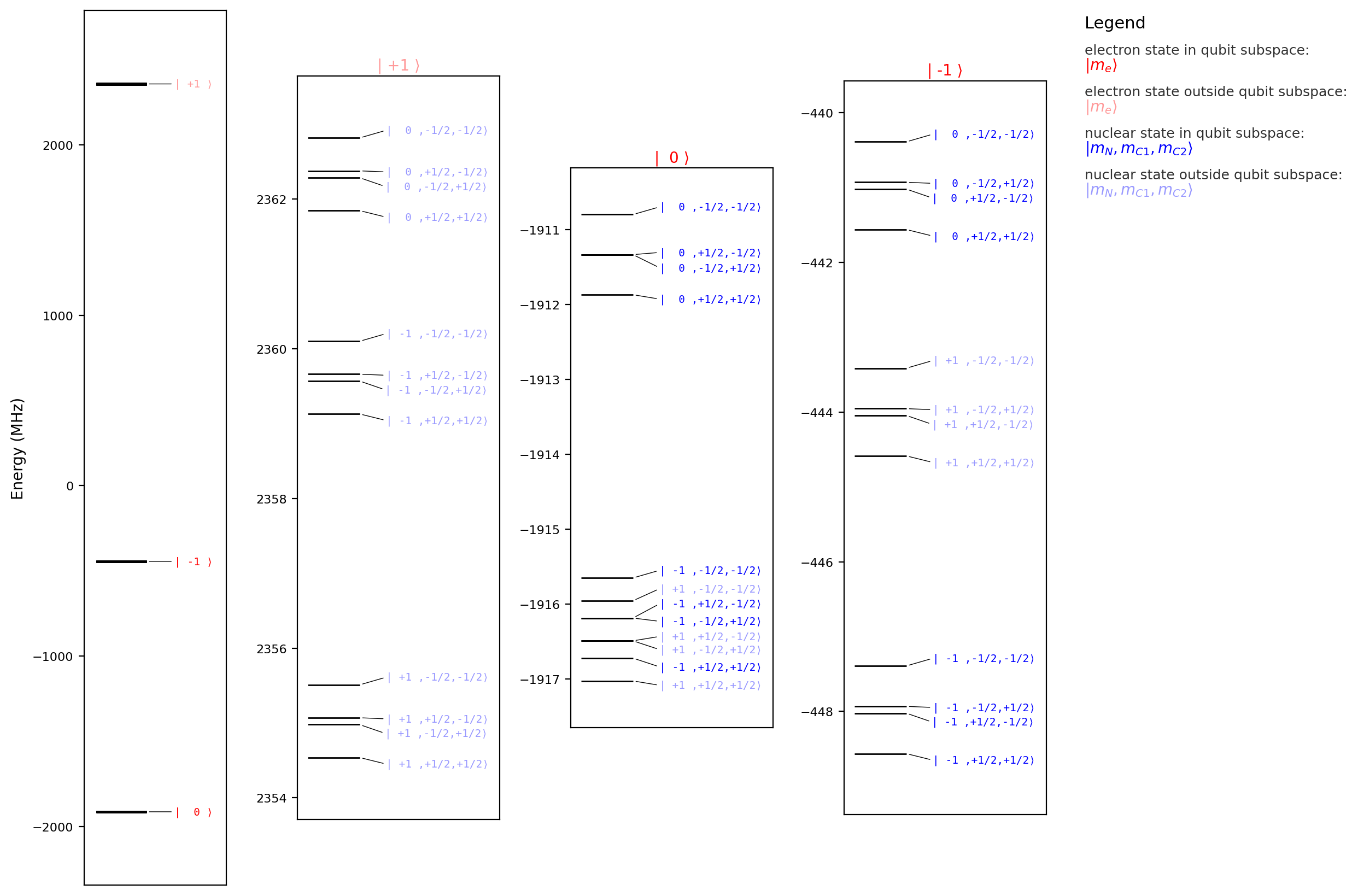
['e', 'N', 'C1', 'C2']
Phase-gate
The phase gate is implemented with a weak electron-spin drive. The pulse rotates the electron spin by \(2\pi\) only when the nuclear spins are in their qubit state \(\ket{1}\) that results an addition \(\pi\) phase for that computational basis state. In this model, that configuration corresponds to the quantum numbers \(m_I=-1\) for the nitrogen spin and \(m_I=1/2\) for the two carbon spins:
rest_quantum_nums = {'N': -1, 'C1': 1 / 2, 'C2': 1 / 2}
frequency = model.splitting_qubit('e', rest_quantum_nums=rest_quantum_nums)
frequency
1468.1596093930461
The target operation is written below as a three-controlled \(\text{RX}(2\pi)\) gate. On the nuclear-spin subspace, with the electron fixed as an ancilla, this is equivalent to a phase gate:
qc = QuantumCircuit(4)
angle = 2 * np.pi
qc.append(RXGate(angle).control(num_ctrl_qubits=3), [1, 2, 3, 0])
qc.draw()
     ┌────────┐
q_0: ┤ Rx(2π) ├
     └───┬────┘
q_1: ────■─────
         │
q_2: ────■─────
         │
q_3: ────■─────
Since the electron is used as an ancilla prepared in \(\ket{0}\), the relevant figure of merit to optimize is the average gate fidelity on the nuclear-spin subspace with ancilla_state={'e': '0'} (see below).
Rectangular pulse baseline
Before moving to the piecewise-constant envelope optimization, we benchmark the single rectangular-envelope pulse. The pulse frequency is set to be resonant with the electron splitting when the nuclear spins are in the qubit state \(\ket{1}\):
def gate_error_rectangle(duration, model, qc):
    rest_quantum_nums = {'N': -1, 'C1': 1 / 2, 'C2': 1 / 2}
    frequency = model.splitting_qubit('e', rest_quantum_nums=rest_quantum_nums)
    angle = 2 * np.pi
    period_time = 2 * np.pi / angle * duration
    amplitude = model.rabi_amplitude_qubit(
        driving_field_name='MW_x',
        period_time=period_time,
        spin_name='e',
        rest_quantum_nums=rest_quantum_nums,
    )

    model.remove_all_pulses()
    model.driving_field('MW_x').add_rectangle_pulse(
        amplitude=amplitude,
        frequency=frequency,
        phase=0,
        duration=duration,
    )
    result = model.simulate_time_evolution(n_eval=2)
    result.ideal = qc
    return 1 - result.average_gate_fidelity(ancilla_state={'e': '0'})
We now scan the pulse duration over a broad range and compute the corresponding gate error:
durations = np.logspace(0, np.log10(2500), 25)
gate_errors = []
for idx, duration in enumerate(durations):
    gate_errors.append(gate_error_rectangle(duration, model, qc))
    print(f'{idx + 1}/{len(durations)}', end=' ')
gate_errors = np.array(gate_errors)
1/25 2/25 3/25 4/25 5/25 6/25 7/25 8/25 9/25 10/25 11/25 12/25 13/25 14/25 15/25 16/25 17/25 18/25 19/25 20/25 21/25 22/25 23/25 24/25 25/25
The resulting duration dependence is shown below:
plt.plot(durations, gate_errors, '.-')
plt.xlabel('Pulse duration [$\mu$s]')
plt.ylabel('Gate error')
plt.xscale('log')
plt.yscale('log')
plt.grid()
plt.show()
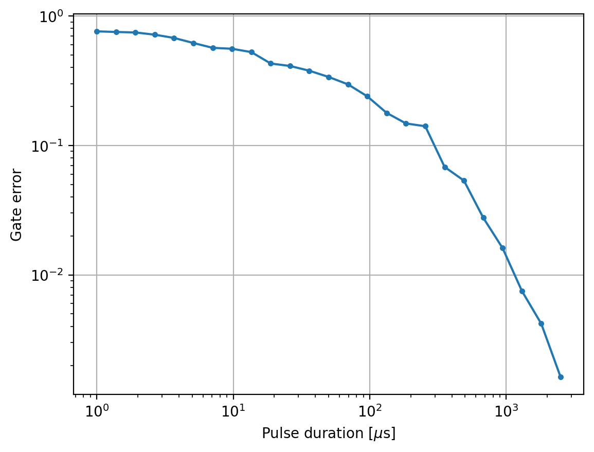
The plot shows that a rectangular pulse reaches low gate error only for relatively long pulse durations, typically above about 1000 \(\mu\)s in this setup.
Optimization helpers
To optimize a pulse with a piecewise-constant envelope using autodiff, we use a bounded parameterization. The pulse-segment amplitudes are mapped from a finite interval to an unconstrained space, optimized there, and then mapped back before the simulation is evaluated.
def bound_to_free(params, bounds):
    def two_sided_bound(x, x_min, x_max):
        scaled_x = 2 * (x - x_min) / (x_max - x_min) - 1
        return jnp.arctanh(scaled_x)

    def two_sided_bound_inv(y, x_min, x_max):
        scaled_y = jnp.tanh(y)
        return (scaled_y + 1) / 2 * (x_max - x_min) + x_min

    free_params = []
    bound_fns = []

    for param, (lower, upper) in zip(params, bounds):
        free_params.append(two_sided_bound(param, lower, upper))
        bound_fns.append(lambda y, lb=lower, ub=upper: two_sided_bound_inv(y, lb, ub))

    def free_to_bound(values):
        return jnp.array([fn(value) for fn, value in zip(bound_fns, values)])

    return jnp.array(free_params), free_to_bound


def optimize_pulse(gate_error, model, init_parameters, bounds, maxiter=100):
    free_parameters, free_to_bound = bound_to_free(init_parameters, bounds)

    def gate_error_free(free_parameters, model):
        return gate_error(free_to_bound(free_parameters), model)

    gate_error_free_value_and_grad = value_and_grad(gate_error_free)
    init_value = gate_error(init_parameters, model)
    opt_result = {'value': [init_value], 'parameters': [init_parameters], 'grad': [jnp.nan]}

    fig, ax = plt.subplots(1, 1)
    ax.set_xlabel('Number of steps')
    ax.set_ylabel('Gate error')
    ax.set_yscale('log')
    ax.xaxis.set_major_locator(MaxNLocator(integer=True))
    ax.grid(visible=True)
    line, = ax.plot(opt_result['value'], 'o-')
    ax.set_xlim(-0.5, 0.5)
    ax.set_xticks([0])
    display(fig)

    state = {'current': None}

    def objective(free_parameters, model):
        value, grad = gate_error_free_value_and_grad(free_parameters, model)
        parameters = free_to_bound(free_parameters)
        state['current'] = (value, parameters, grad)
        return value, grad

    def refresh_plot(values):
        line.set_data(range(len(values)), values)
        if len(values) == 1:
            ax.set_xlim(-0.5, 0.5)
            ax.set_xticks([0])
        else:
            ax.set_xlim(-0.5, len(values) - 0.5)
            ax.xaxis.set_major_locator(MaxNLocator(integer=True))
            ax.relim()
            ax.autoscale_view(scalex=False, scaley=True)
        clear_output(wait=True)
        display(fig)

    def callback(_):
        value, parameters, grad = state['current']
        opt_result['value'].append(value)
        opt_result['parameters'].append(parameters)
        opt_result['grad'].append(grad)
        refresh_plot(opt_result['value'])

    res = minimize(
        fun=objective,
        args=model,
        x0=free_parameters,
        jac=True,
        method='L-BFGS-B',
        options={'gtol': 1e-12, 'ftol': 1e-12, 'maxiter': maxiter},
        callback=callback,
    )
    opt_result['res'] = res
    plt.close(fig)
    return opt_result
To set the pulse amplitude scale, we define an upper bound based on a maximum allowed electron-spin Rabi frequency:
max_rabi_frequency = 500 # MHz
max_duration = 0.5 / max_rabi_frequency
max_amplitude = model.rabi_amplitude_qubit(
    driving_field_name='MW_x',
    period_time=2 * max_duration,
    spin_name='e',
)
Piecewise-constant pulse-envelope optimization
We now switch from a single rectangular-envelope pulse to a piecewise-constant complex envelope. The pulse is represented by n complex samples with a fixed time step dt, and the real and imaginary parts are optimized as independent parameters:
frequency = model.splitting_qubit('e', rest_quantum_nums={'N': -1, 'C1': 1 / 2, 'C2': 1 / 2})

def gate_error_discrete(parameters, model, n_shots=1, n_split=101):
    samples = jnp.array(parameters[0::2]) + 1j * jnp.array(parameters[1::2])

    model.remove_all_pulses()
    model.driving_field('MW_x').add_discrete_pulse(
        samples=samples,
        frequency=frequency,
        dt=dt,
    )

    result = model.simulate_time_evolution(n_eval=2, n_shots=n_shots, n_split=n_split)
    result.ideal = qc
    return 1 - result.average_gate_fidelity(ancilla_state={'e': '0'})
The total pulse duration is set to \(125\,\mu\mathrm{s}\) and divided into 25 equal segments, resulting in 50 optimized parameters. The optimization is initialized with a randomized complex pulse. The initial segment amplitudes are sampled around the Rabi amplitude of the corresponding rectangular pulse, while the phases are chosen uniformly at random:
duration = 125
n = 25

rest_quantum_nums = {'N': -1, 'C1': 1 / 2, 'C2': 1 / 2}
amplitude = model.rabi_amplitude_qubit(
    driving_field_name='MW_x',
    period_time=duration,
    spin_name='e',
    rest_quantum_nums=rest_quantum_nums,
)
dt = duration / n

samples = []
for _ in range(n):
    a = amplitude * np.random.uniform(0.5, 1.5)
    phi = np.random.uniform(0, 2 * np.pi)
    samples.append(a * np.cos(phi))
    samples.append(a * np.sin(phi))

params = jnp.array(samples)
bounds = [(-max_amplitude, max_amplitude) for _ in range(2 * n)]
With the model, target gate, objective, and initialization in place, we can run the pulse optimization. The plot is updated after each optimization step:
opt_result = optimize_pulse(
    gate_error_discrete,
    model,
    params,
    bounds,
    maxiter=100,
)
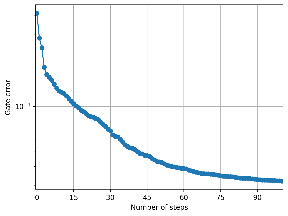
The final gate fidelity exceeds \(99.9\%\), which is a remarkably good result, especially considering that a rectangular pulse of the same duration achieves a fidelity of only around \(90\%\):
final_gate_error = opt_result['value'][-1]
1 - final_gate_error
Array(0.96794268, dtype=float64)
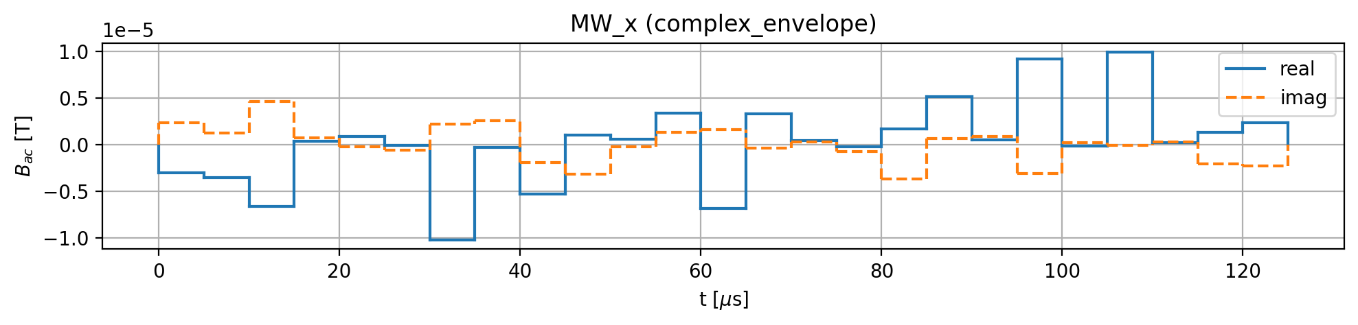
The resulting optimized pulse sequence is shown below:
model.driving_field('MW_x').plot_pulses(function='complex_envelope')
Note: This optimization process is conceptually similar to the Gradient Ascent Pulse Engineering (GRAPE) method, but it does not rely on the rotating wave approximation (RWA) and explicitly accounts for leakage outside the computational subspace.